|
|
I. Mathematical methods of gauge theory
A.
Differential forms
Monday, January 5,
2009
Lecture: The reason for gauge theory; pictures of
fiber bundles; the wedge product.
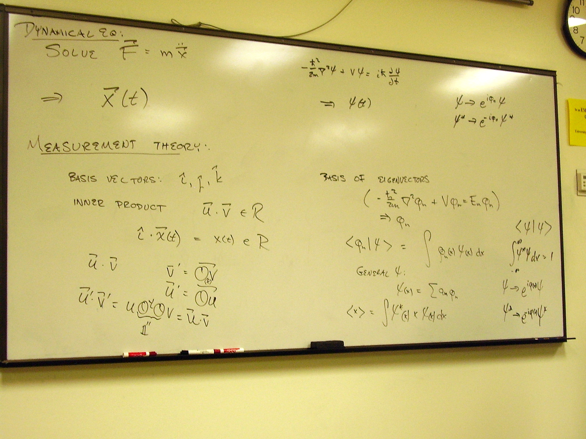
The reason for gauge theory:
the symmetry of dynamical equations is typically global, while the symmetry of
the corresponding measurement theory is usually local. Gauge theory is a means
of extending the symmetry of a set of dynamical equations to match that of the
measurement theory, thus providing the maximal measurable information.
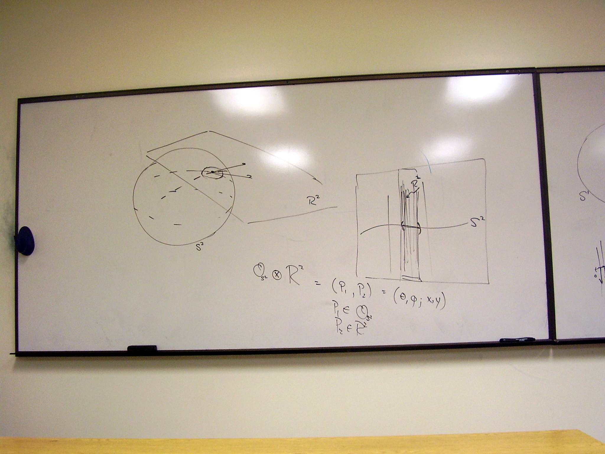
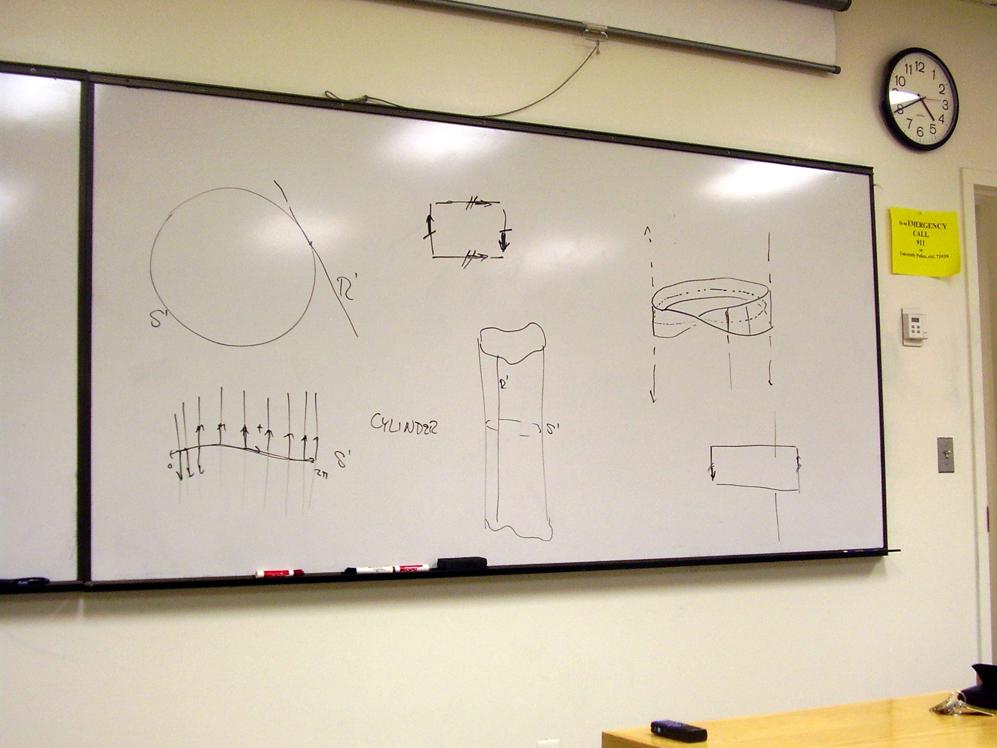
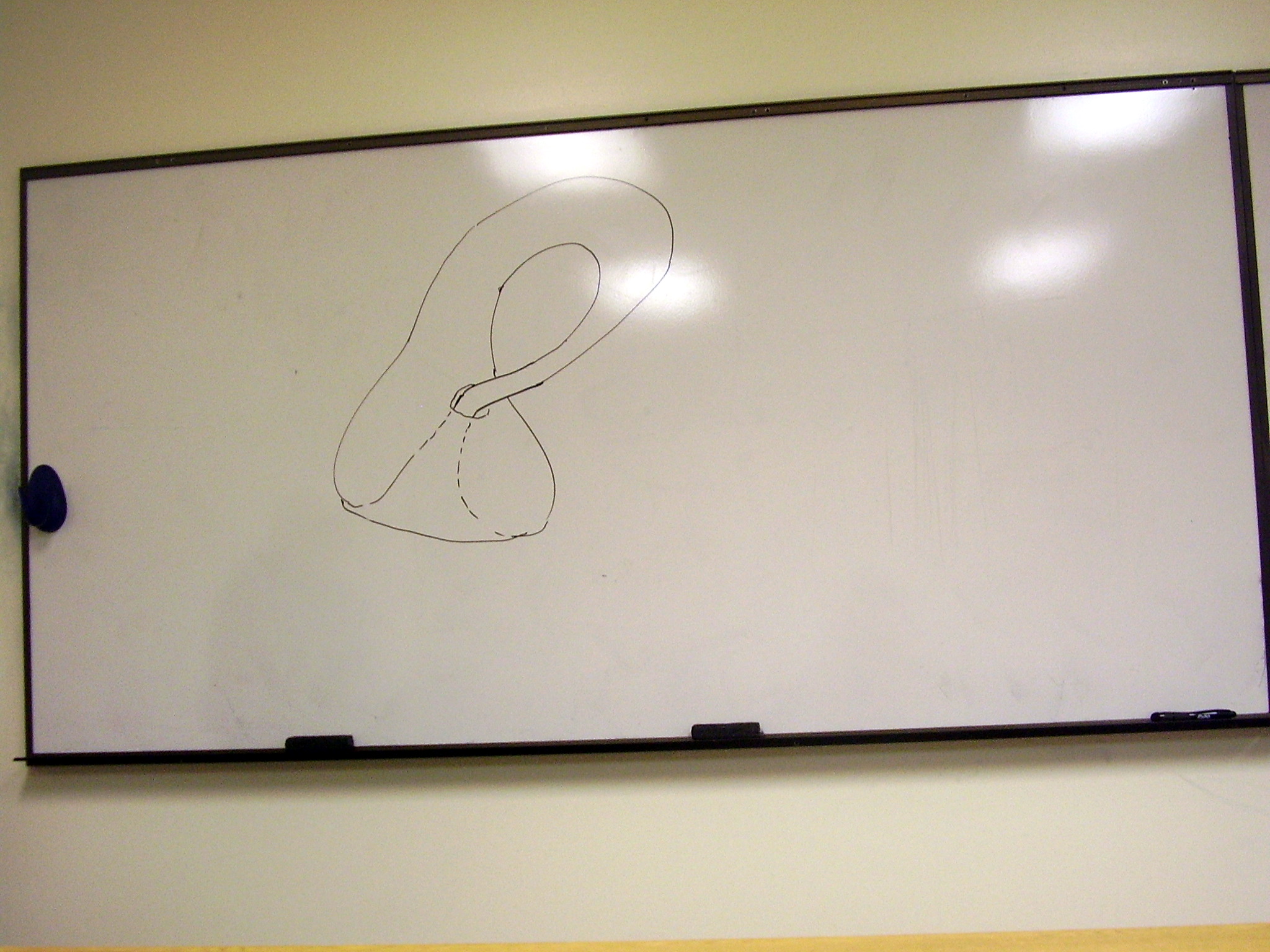
Fiber bundles are used to
describe local symmetries. Some pictures of simple fiber bundles: Tangent
bundle of a sphere; Cylinder vs. Mobius strip; (sphere) vs. Klein bottle:
Beginning differential
forms: the wedge product
A better Klein bottle:
Klein Bottle (from Wikimedia, en.wikipedia.org/ wiki/Klein_bottle)
Wednesday, January 7,
2009
Lecture:
Practice with the wedge product. The exterior derivative.
Finding the dimension of the
space of p-forms
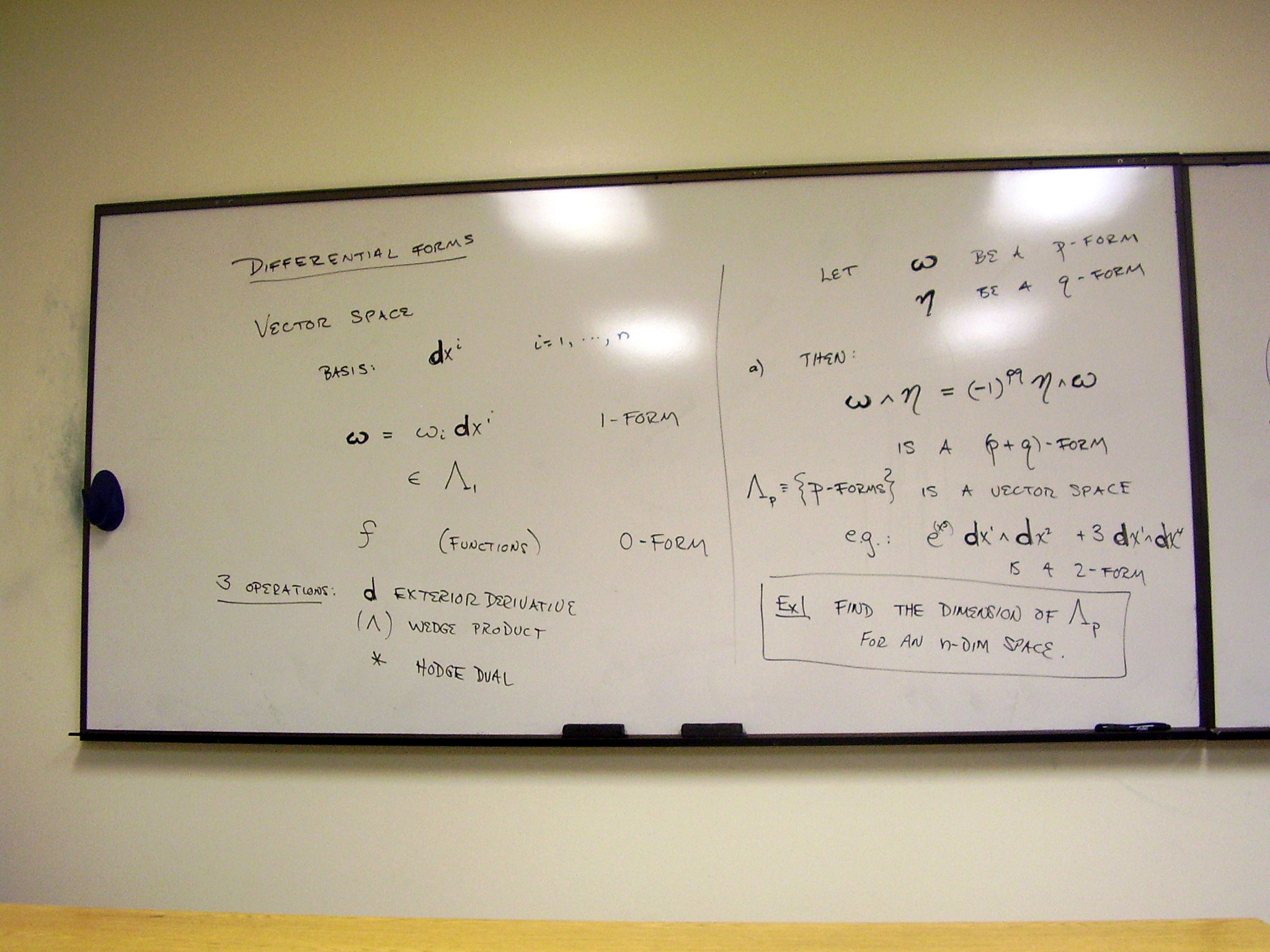
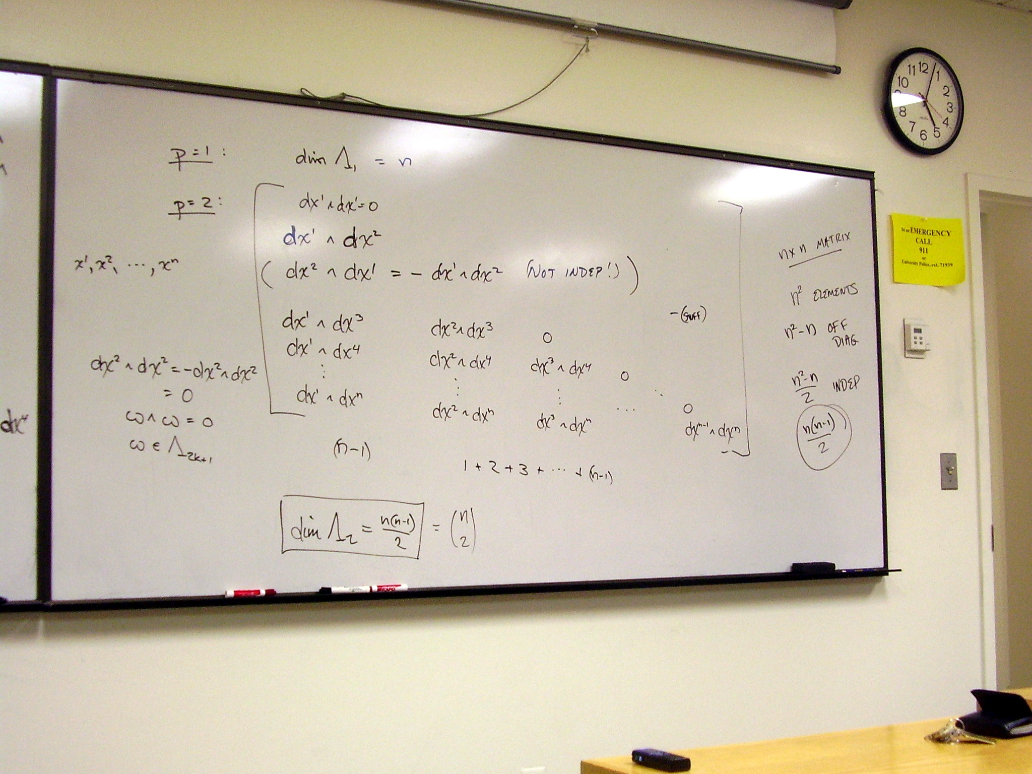
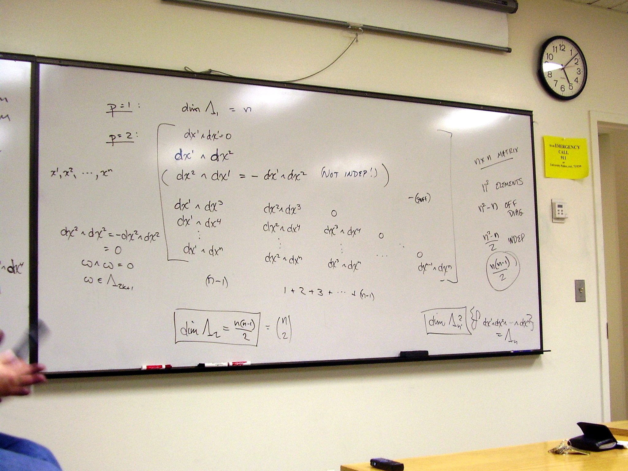
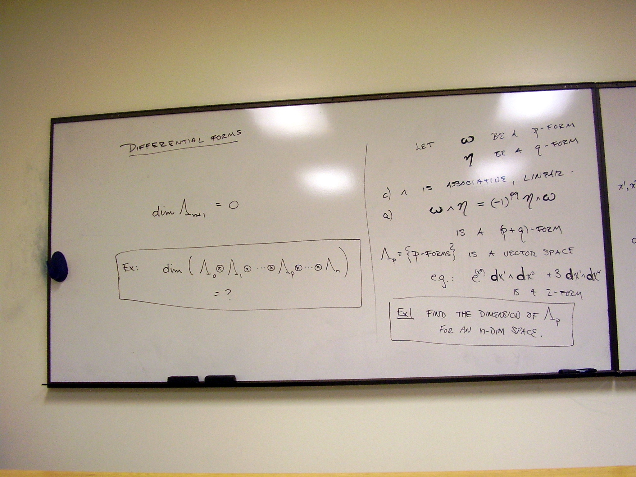
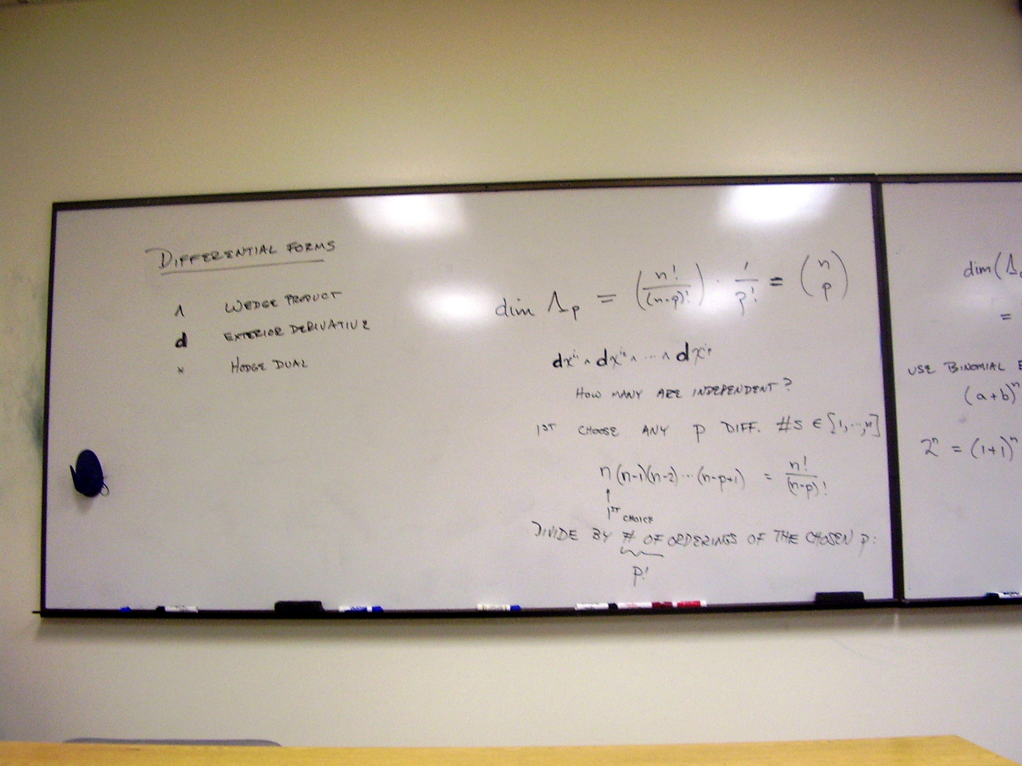
Finding the dimension of the
space of forms
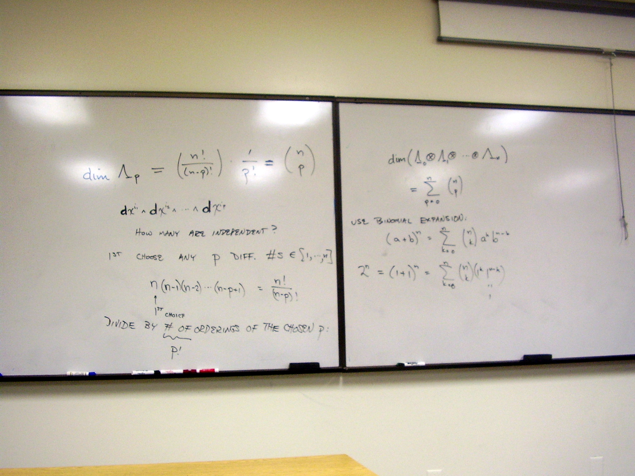
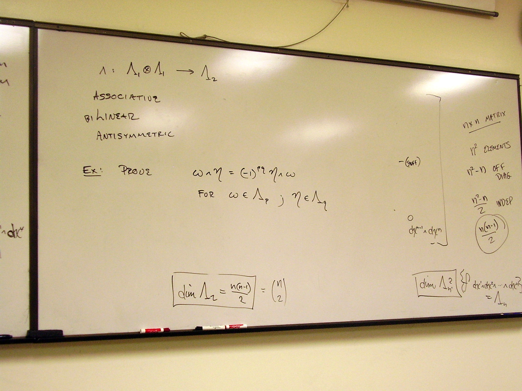
Example: commuting forms
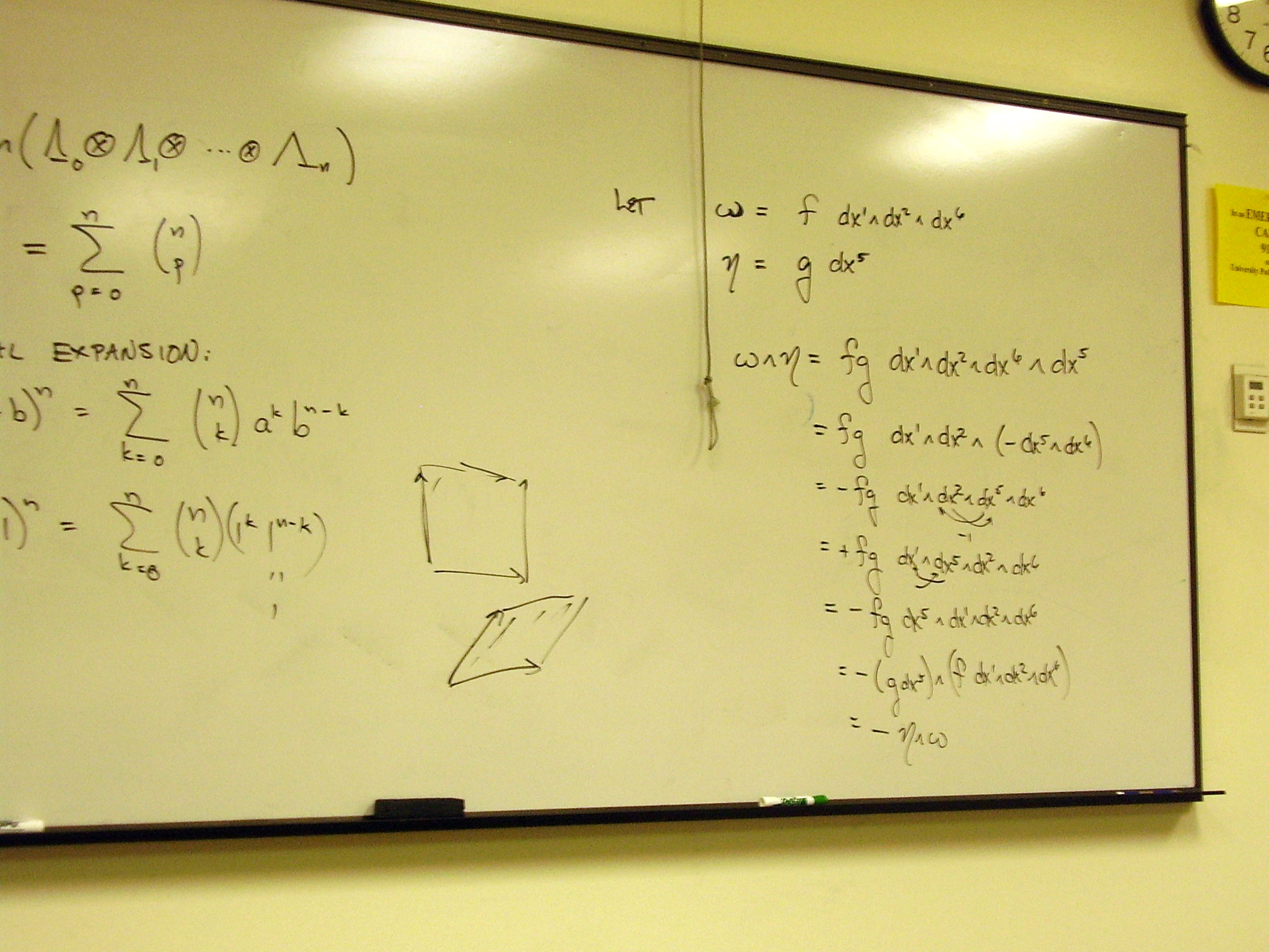
Examples: Write out all
p-forms when n = 3. Exercises
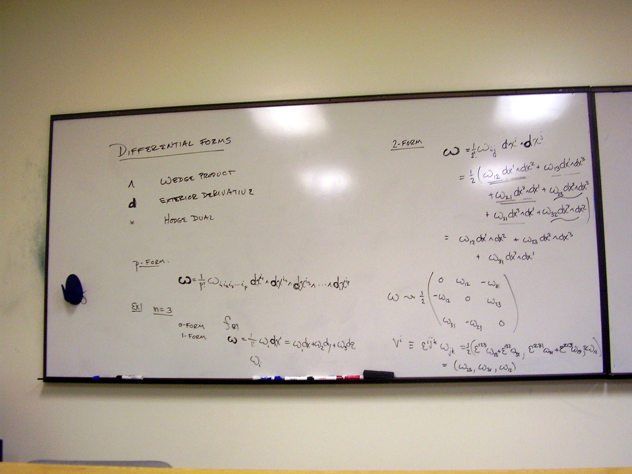
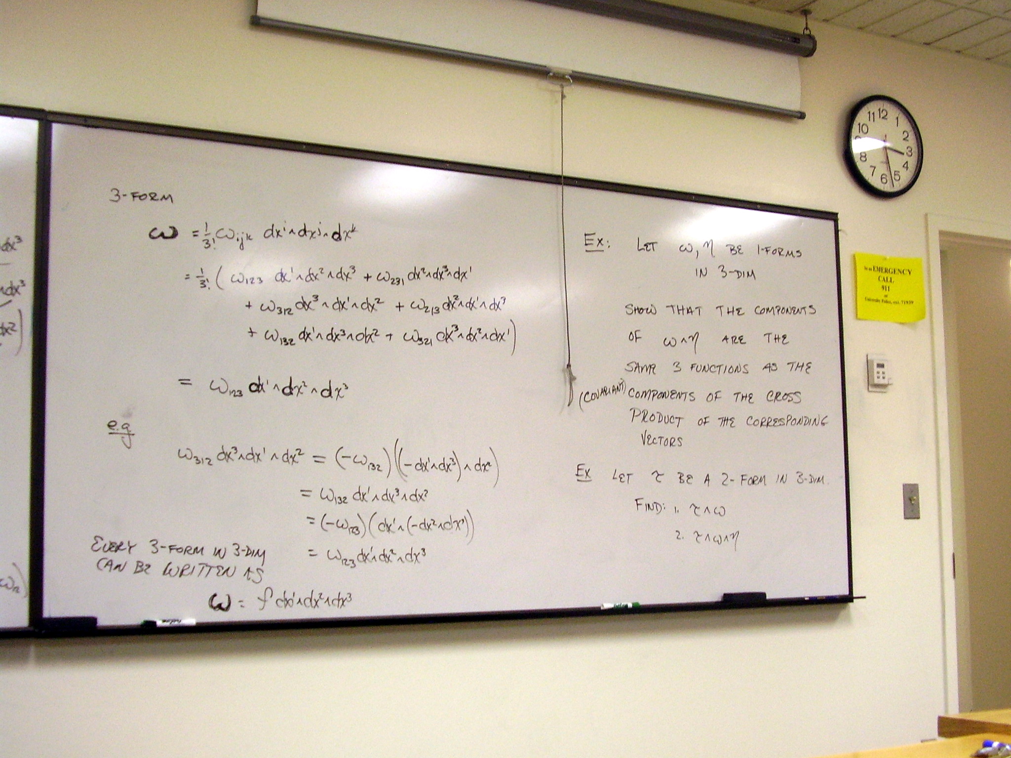
The exterior derivative of a
0-form; the exterior derivative of a 1-form
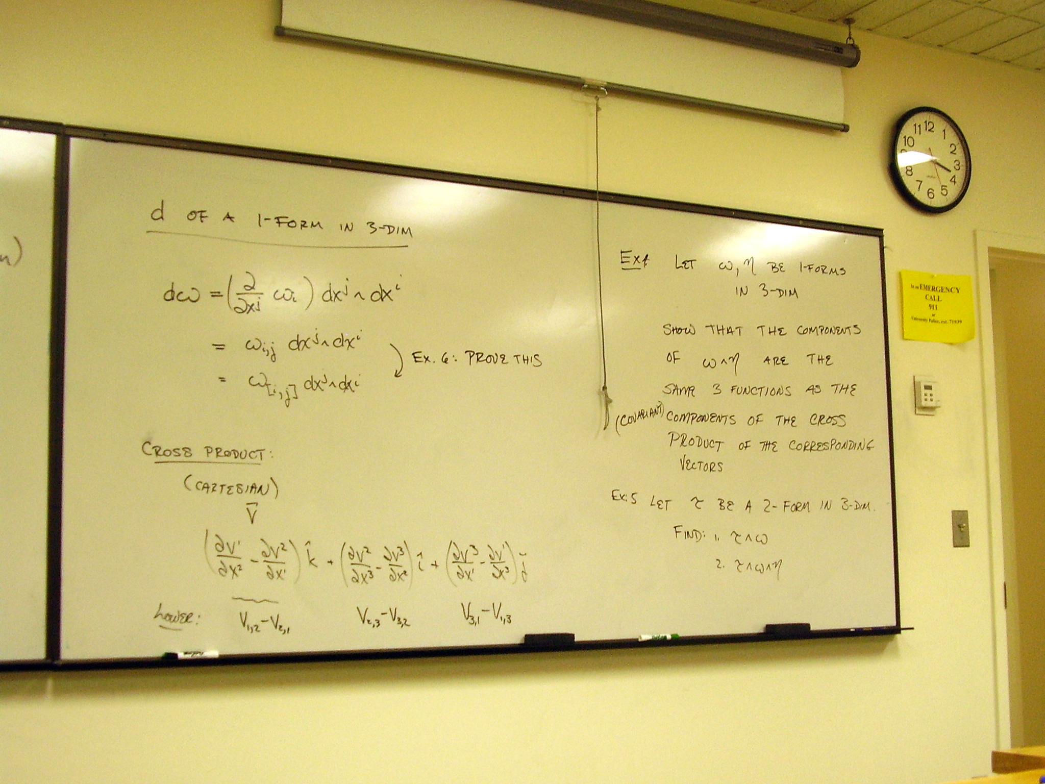
Exercise.
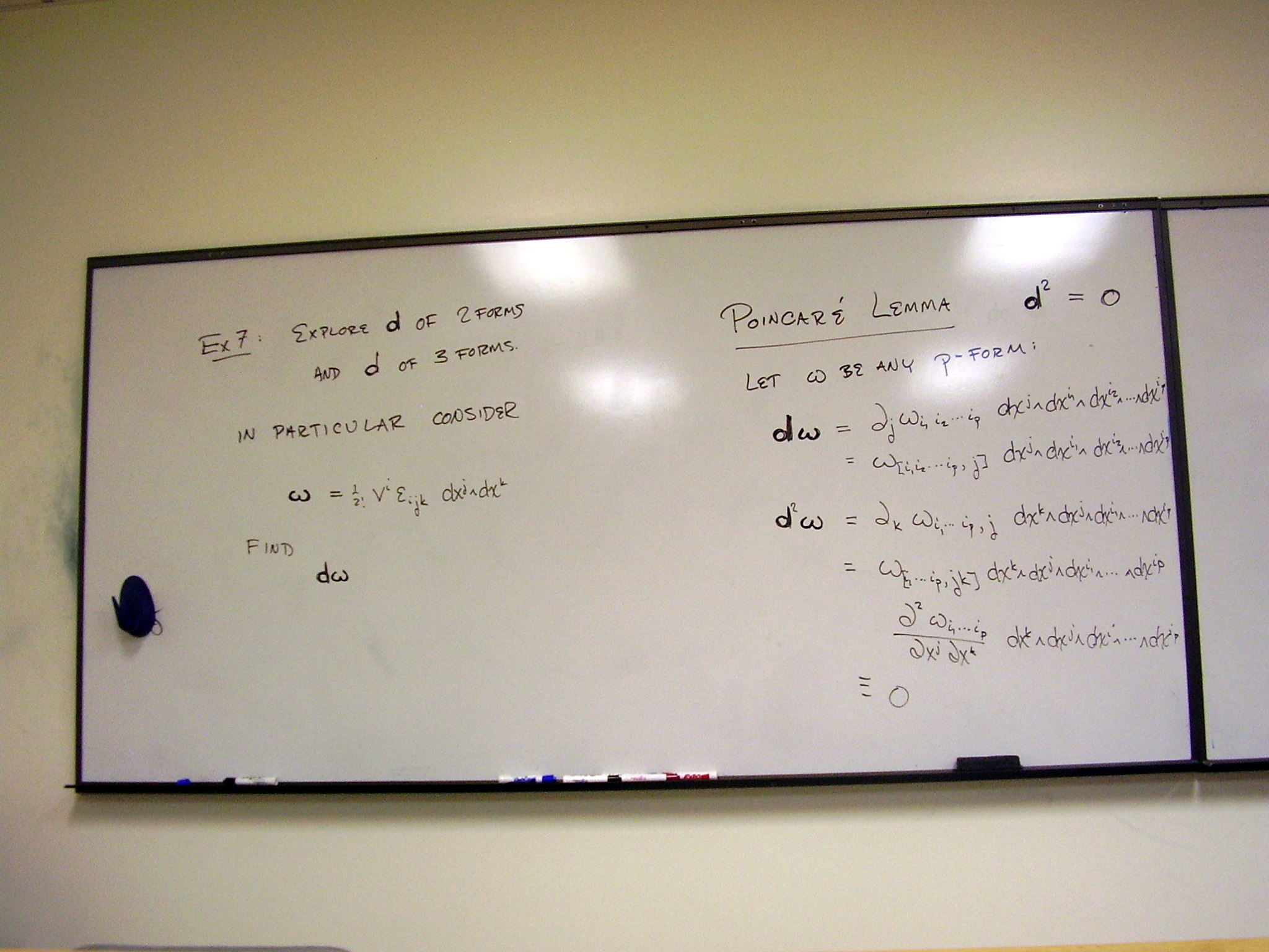
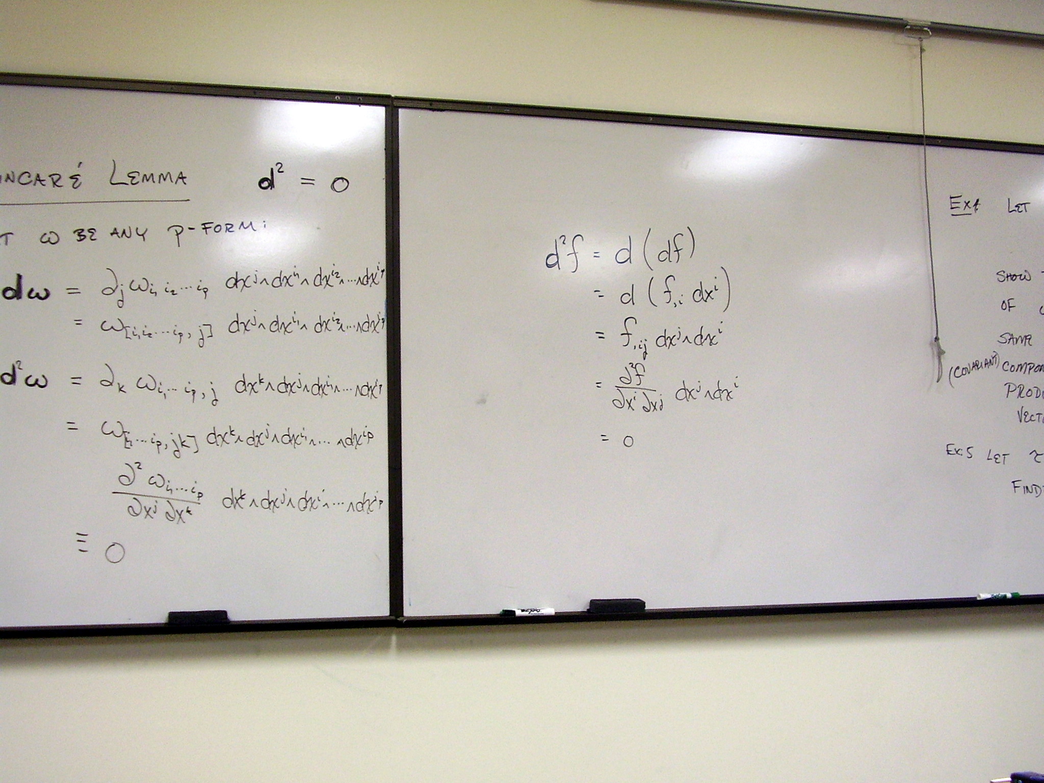
The Poincaré lemma, d2
= 0.
Friday, January 9, 2009
Lecture:
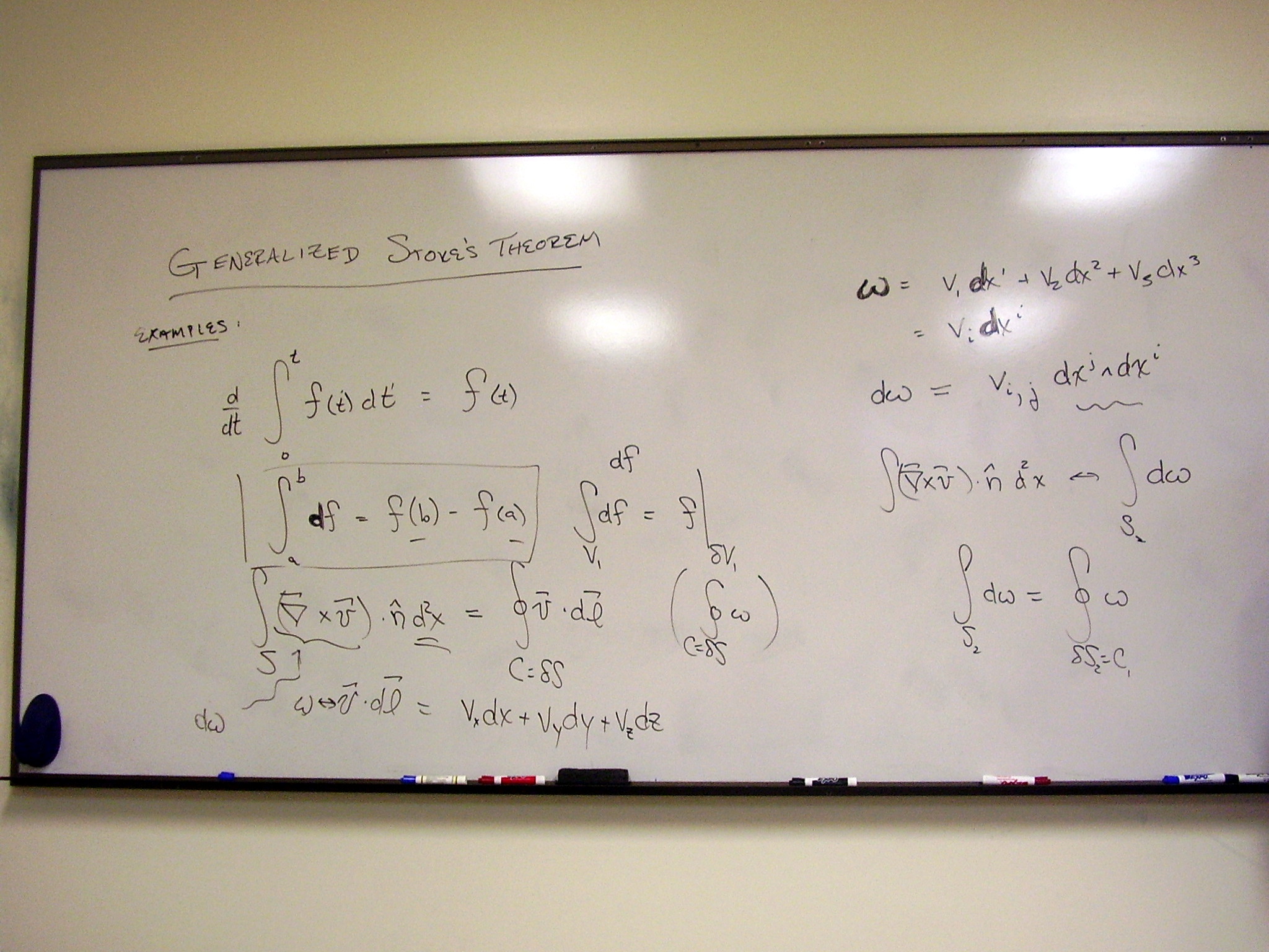
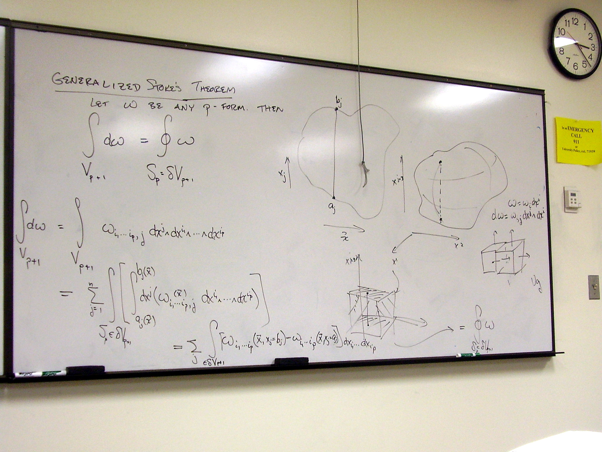
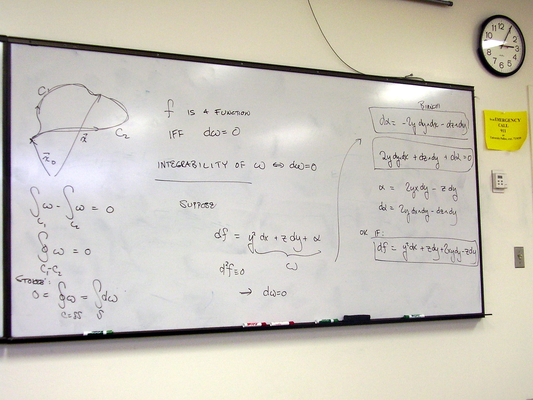
The generalized Stokes theorem and the converse to the Poincaré lemma.
Examples of the generalized
Stokes theorem for 0-forms and 1-forms.
Statement and brief proof of
the generalized Stokes theorem.
The explicit form of Stokes’
theorem for 0- and 1-forms. An exercise.
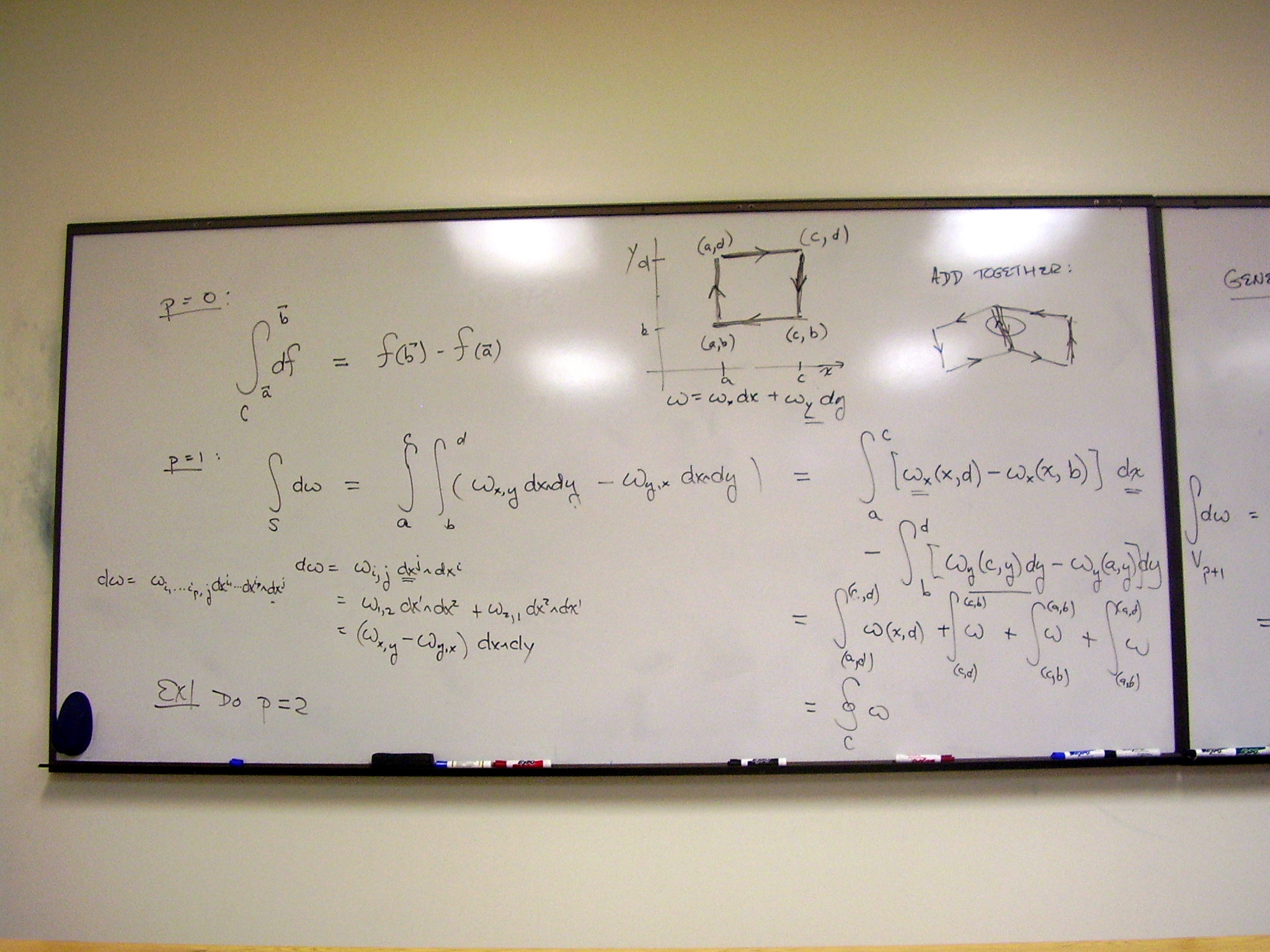
The Poincaré lemma and its
converse. Closed and exact forms.
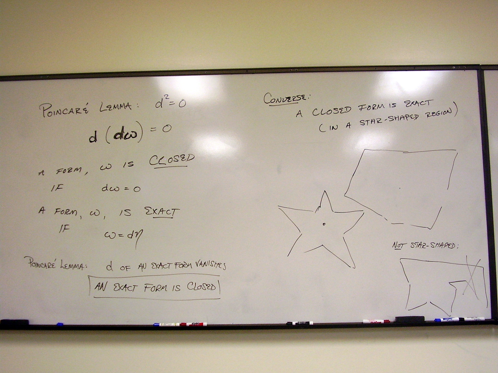
Proof of the converse to the
Poincaré lemma.
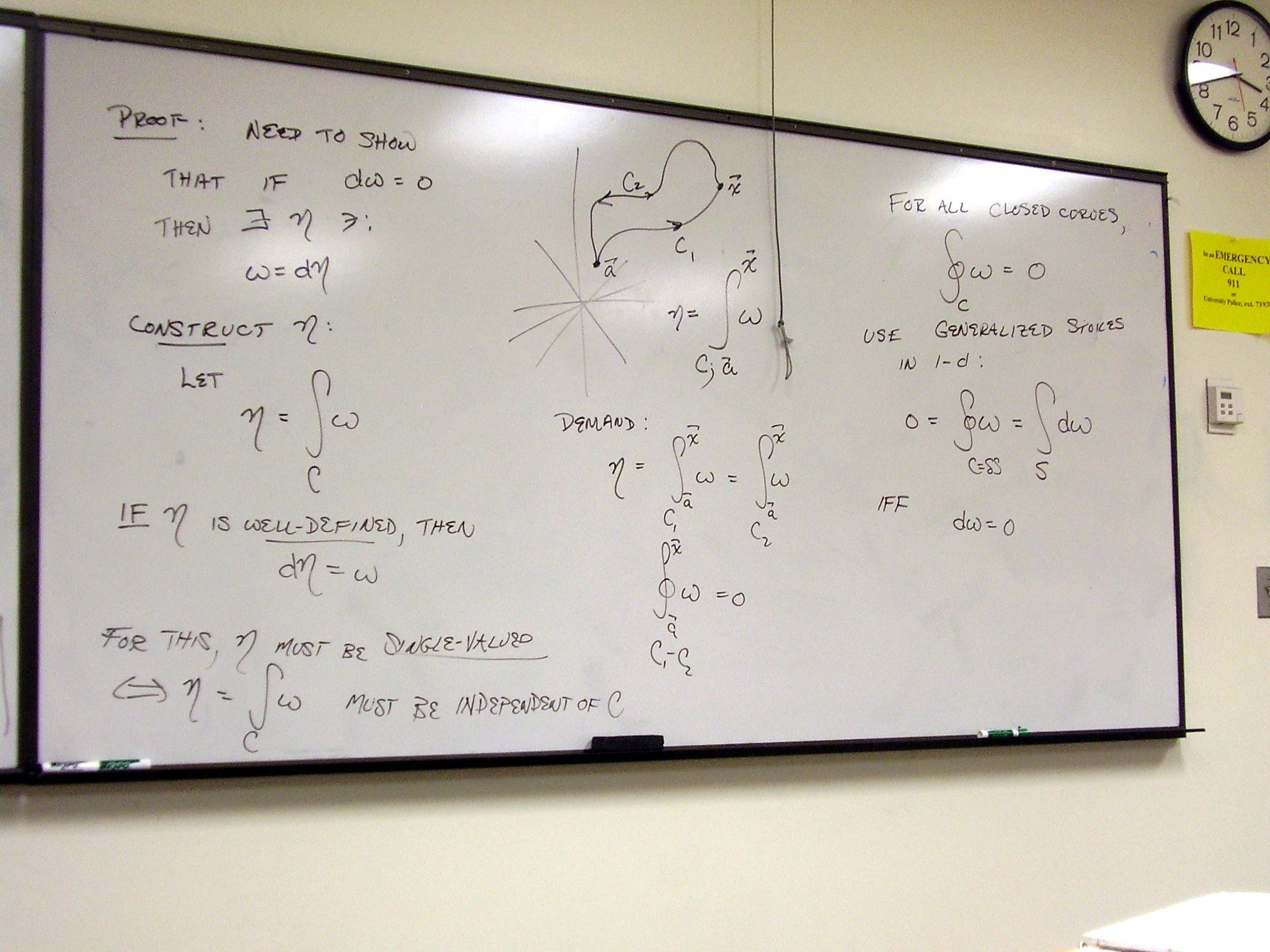
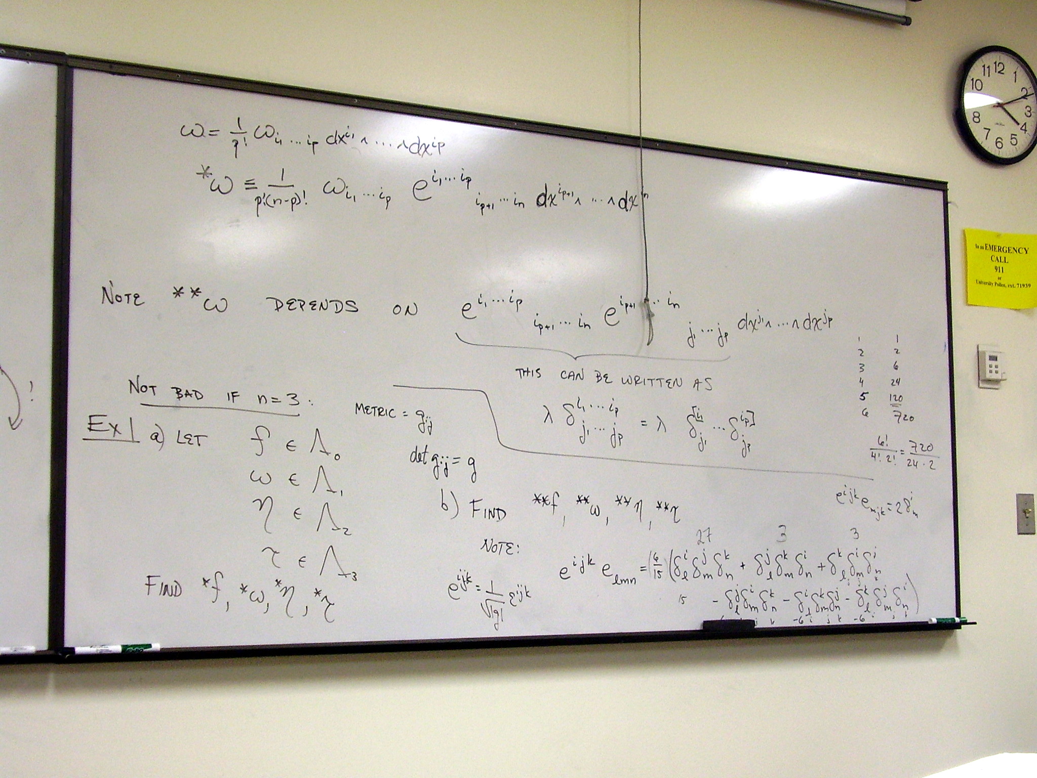
Exercise: an application of
the converse to the Poincaré lemma. Definition of the Hodge dual (star).
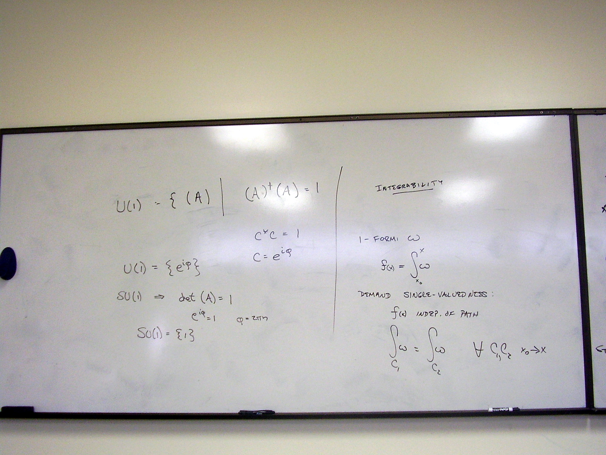
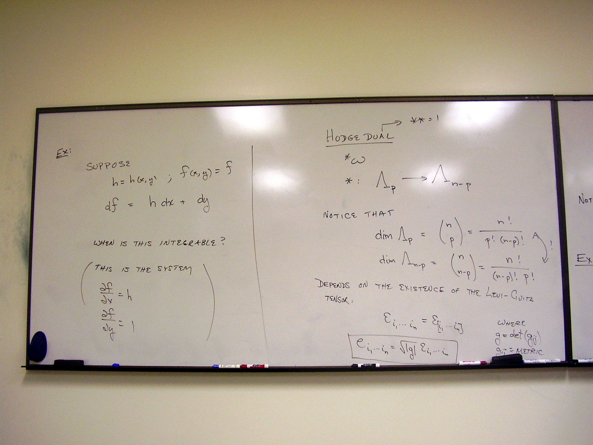
The Hodge dual. Exercises.
Monday, January 12,
2009
Lecture:
The Hodge dual; electromagnetism in differential forms
Definition of the Hodge
dual, or star, operator:
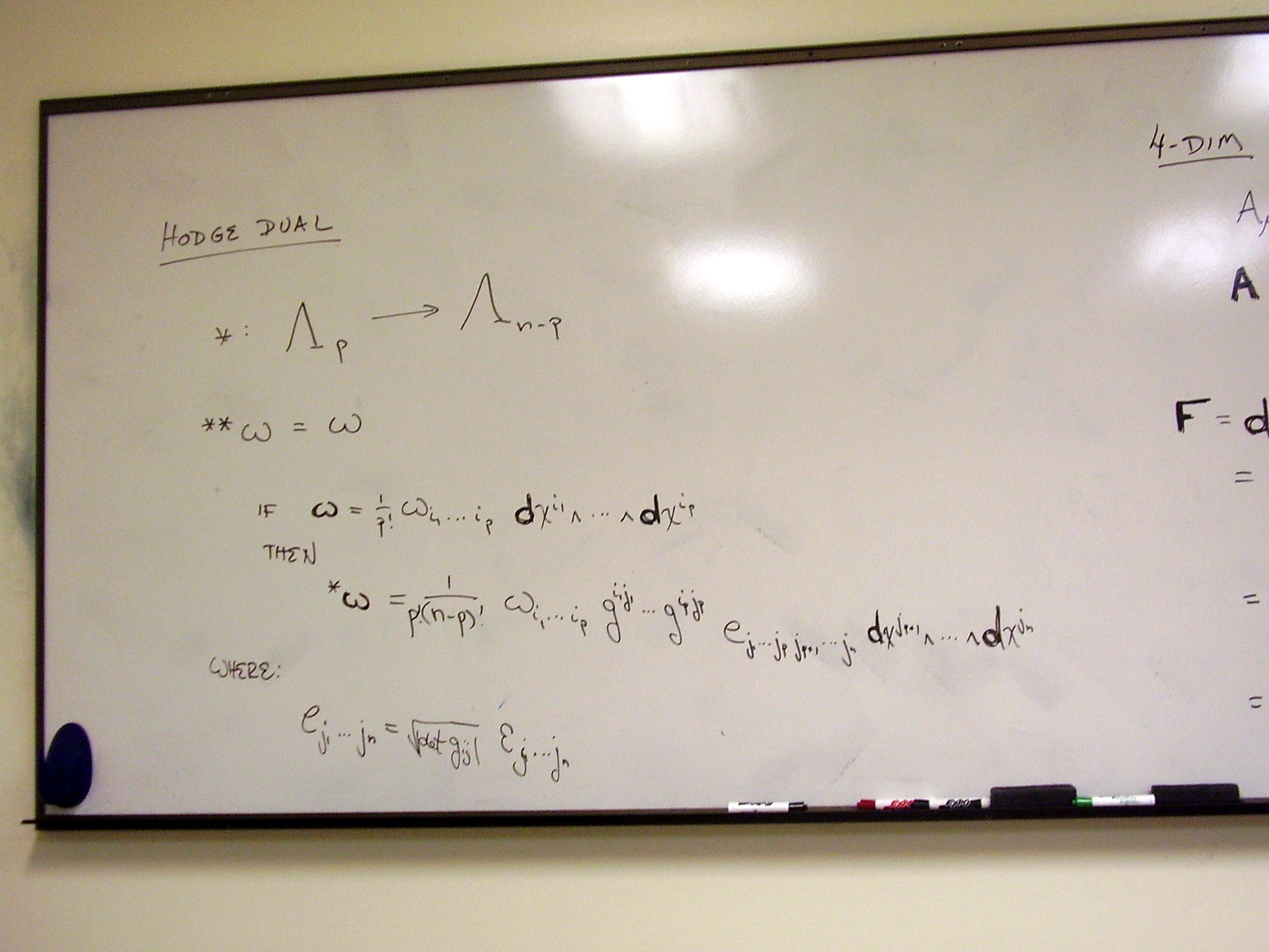
The Maxwell field tensor and
its Hodge dual:
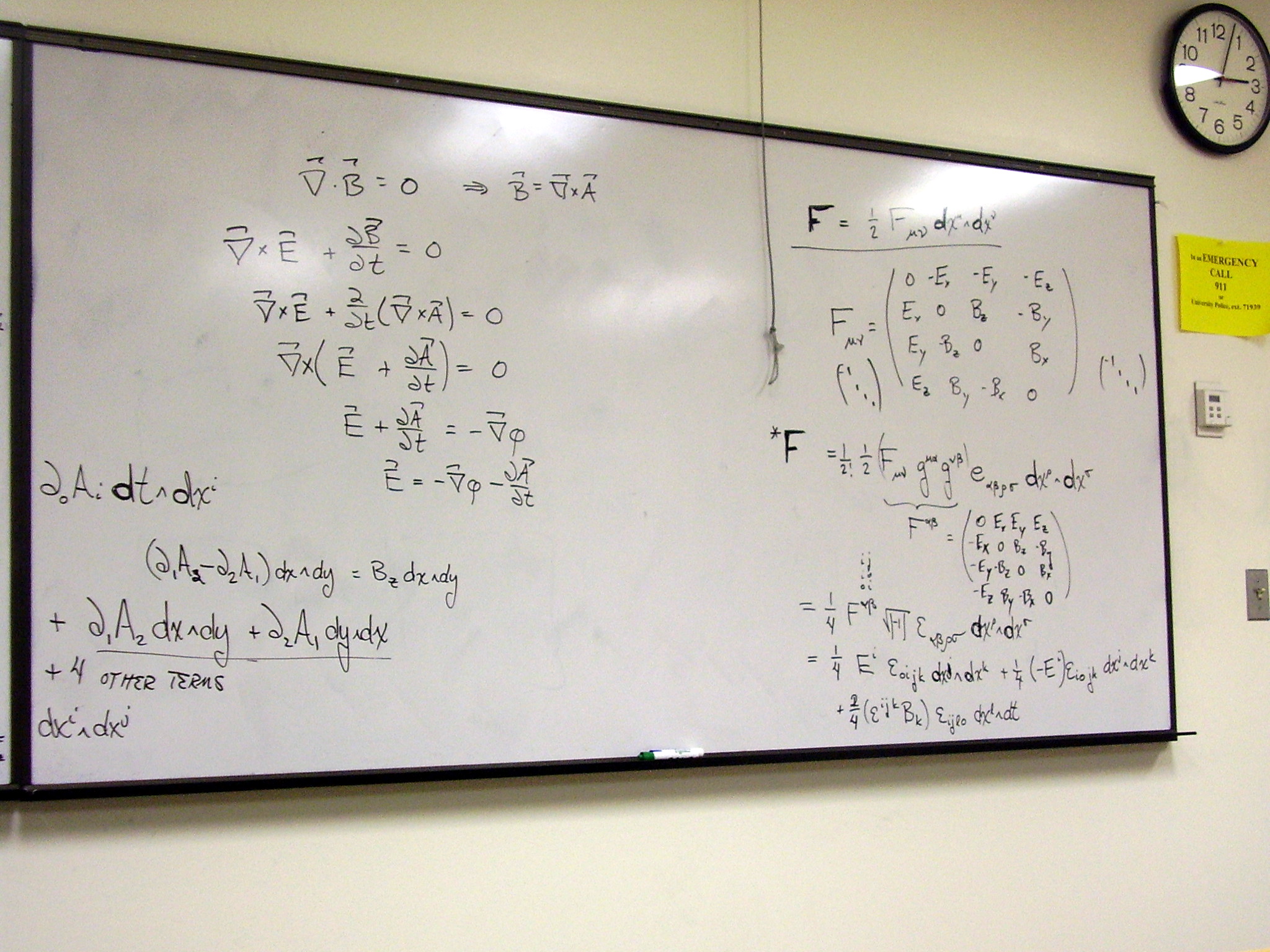
The Hodge duality exchanges
the electric and magnetic fields, with one sign flip. Writing the gradient,
curl and divergence in differential forms. For the gradient, we just take the
components of the exterior derivative of a 0-form, and raise the index. The
curl is more involved.
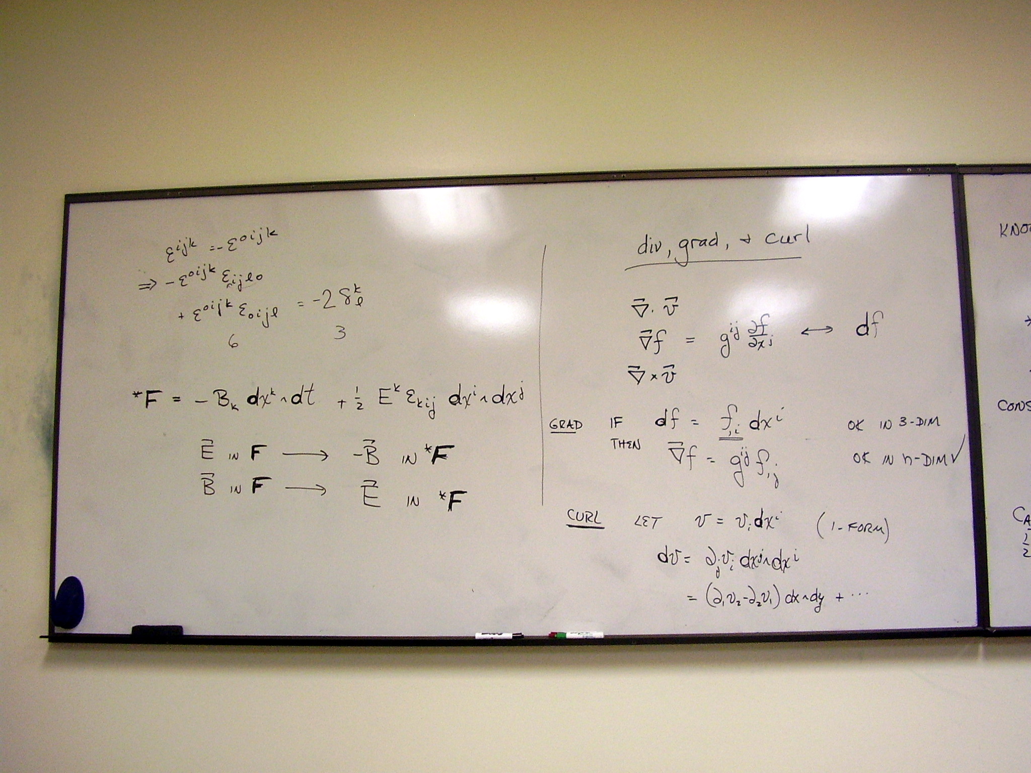
For the curl, we start with
the exterior derivative of a 1-form. This gives a 2-form, which we turn back
into a 1-form by taking the Hodge dual. Finally, raise the free index. Notice
that we can also use the covariant derivative to arrive at the same result.
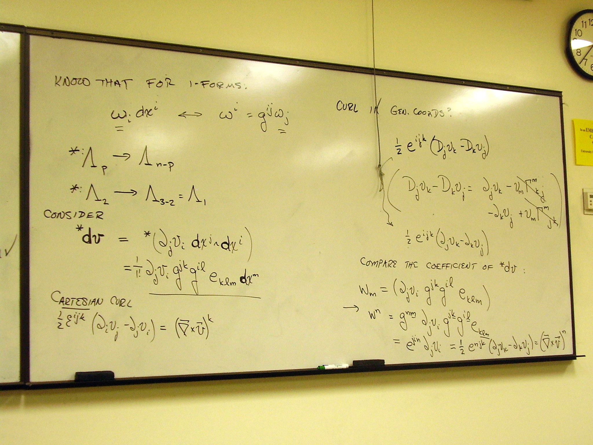
Notice that the covariant
derivative was not required for the gradient, because we are differentiating a
function
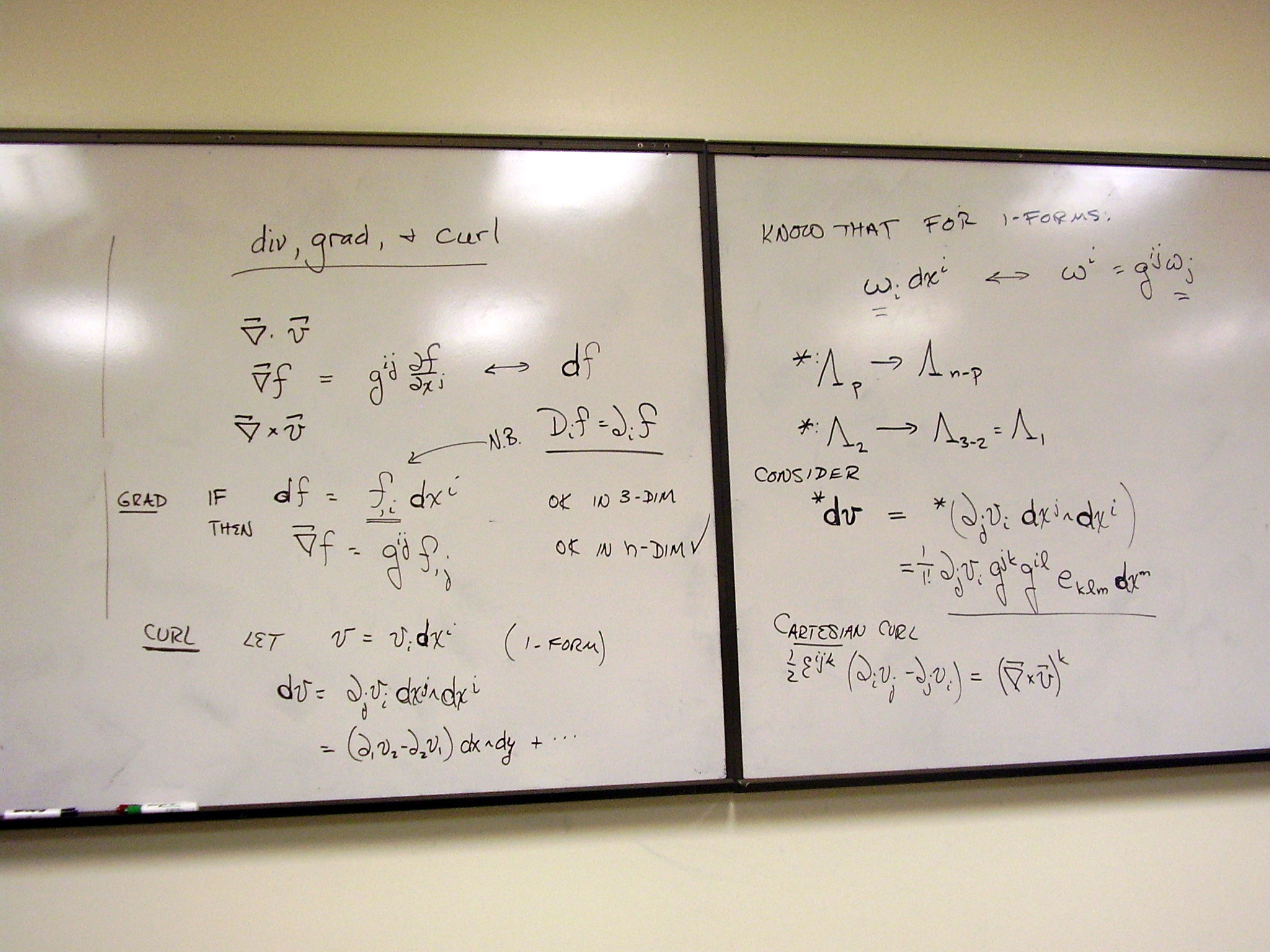
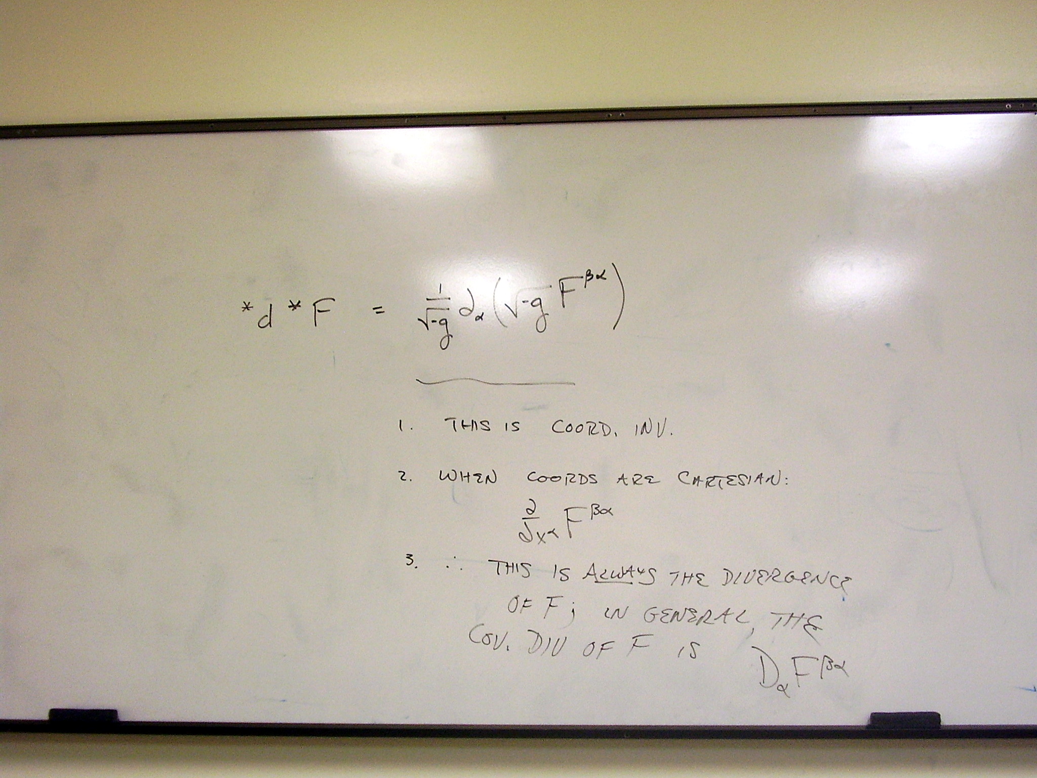
The divergence. Using
differential forms is coordinate invariant. Since the result we get is correct
when the determinant of the metric is 1 (Cartesian coordinates), we can
conclude that we have derived a coordinate invariant generalization of the
usual Cartesian form. This formula is much simpler than brute force change of
coordinates!
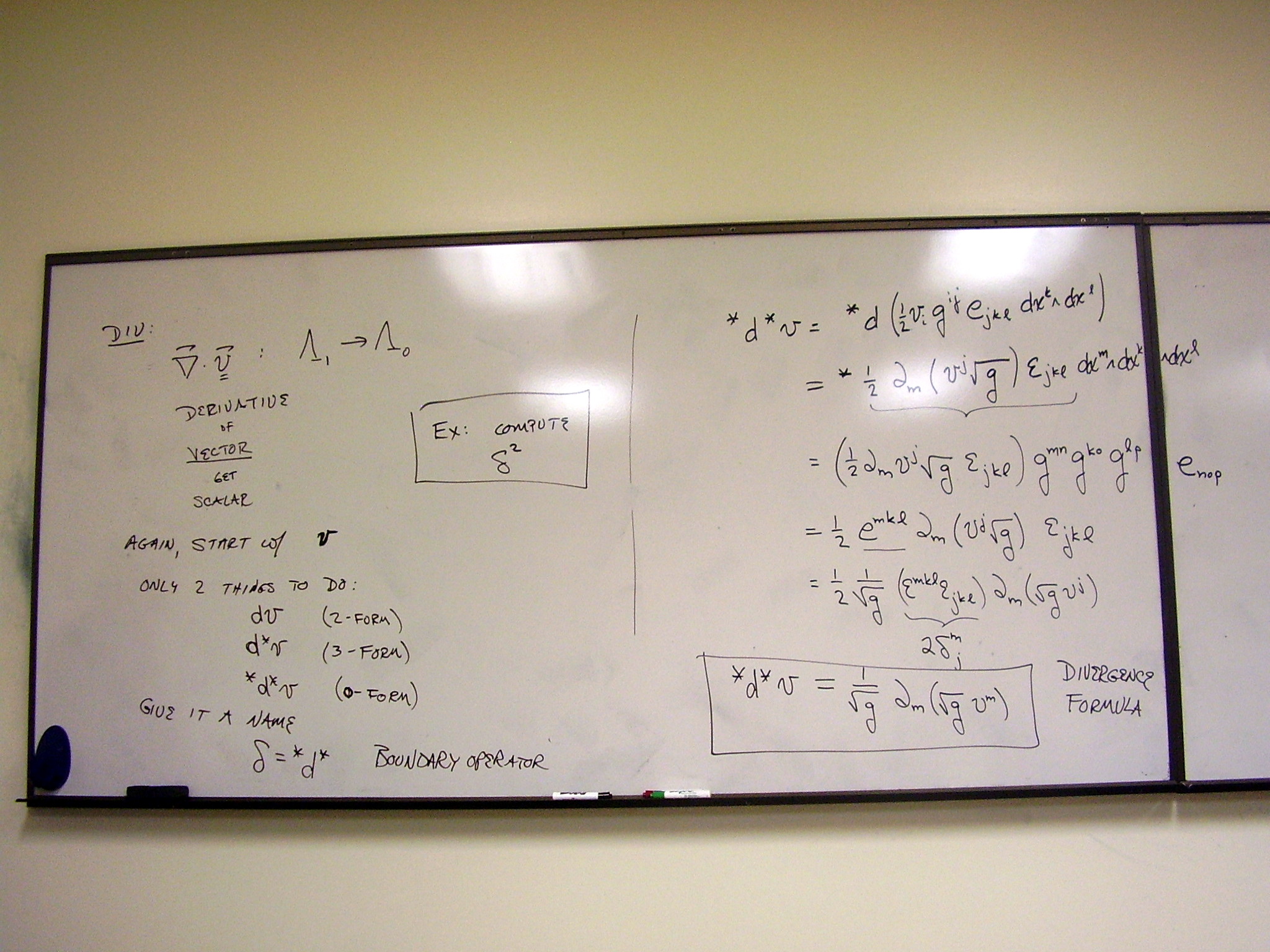
Here’s a way to write the
curl in arbitrary coordinates when given the contravariant components of the
vector.
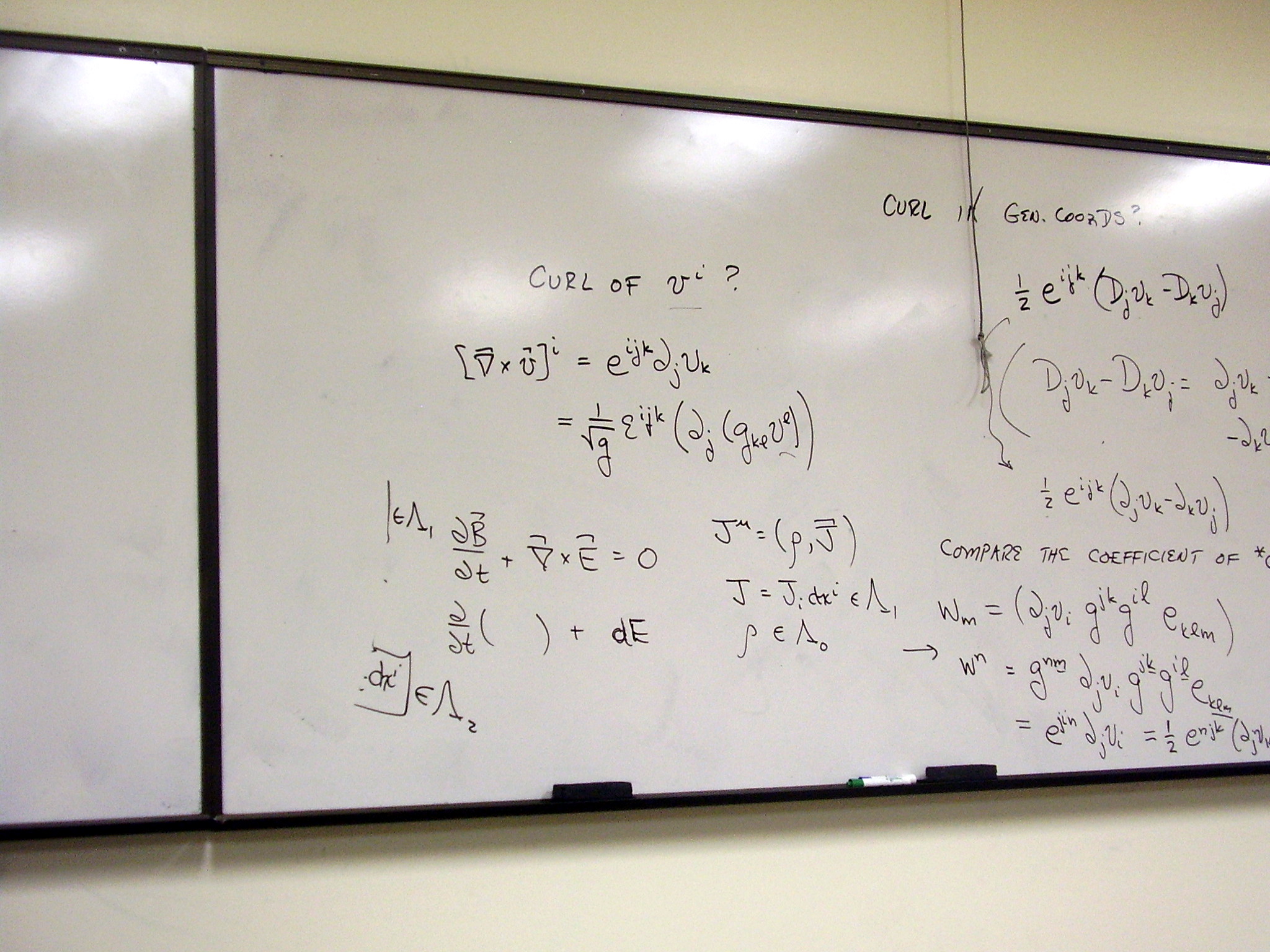
Exercise: 3-d Maxwell
equations
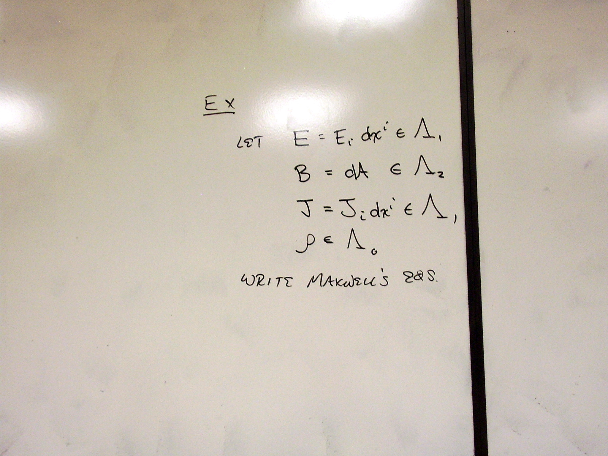
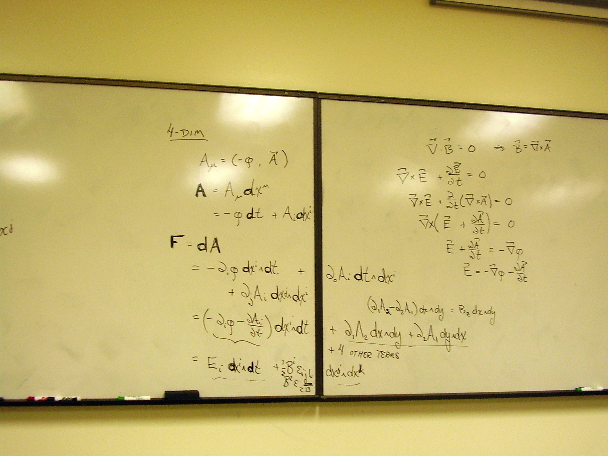
Write the 4-dimensional
version of Maxwell’s equations using differential forms.
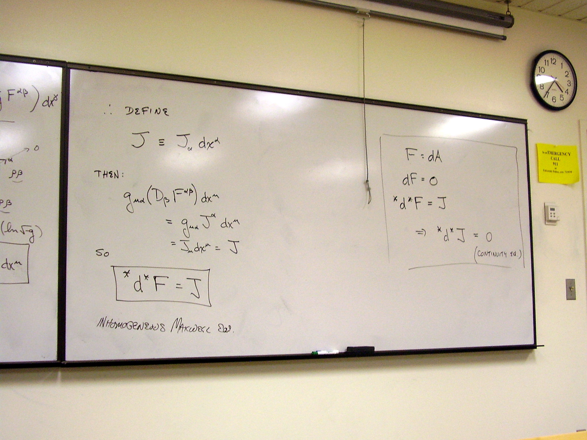
The potential 2-form; the
field tensor is a 2-form. The Poincaré lemma applied to F = dA gives dF = 0. This becomes the two
homogeneous Maxwell equations.
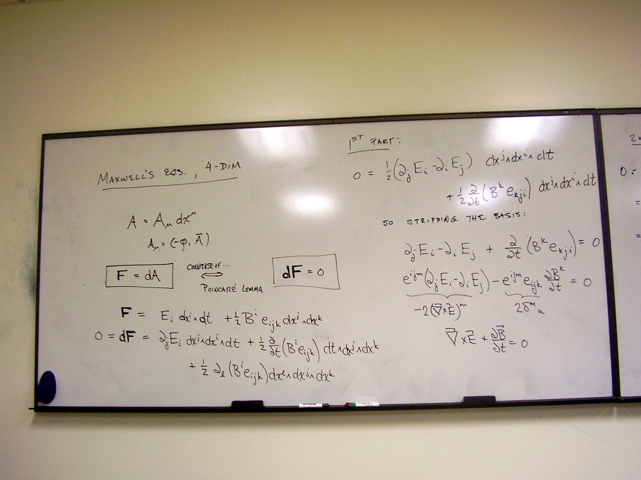
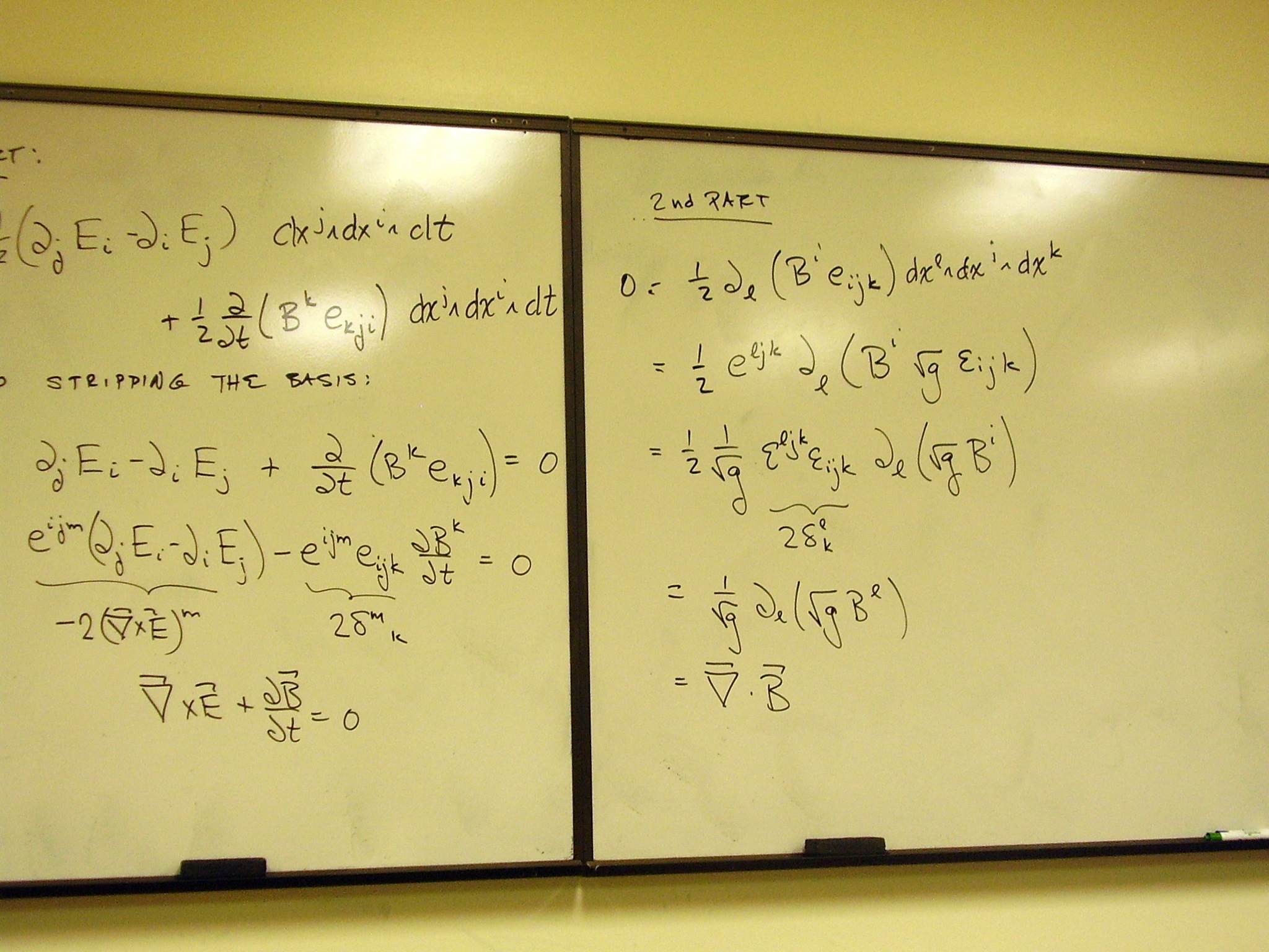
Apply the boundary operator
– i.e., the Hodge dual of the exterior derivative of the Hodge dual
– to the Maxwell field 2-form. Recognize the resulting divergence as the
charge density/current 4-vector. The inhomogeneous Maxwell equations result.
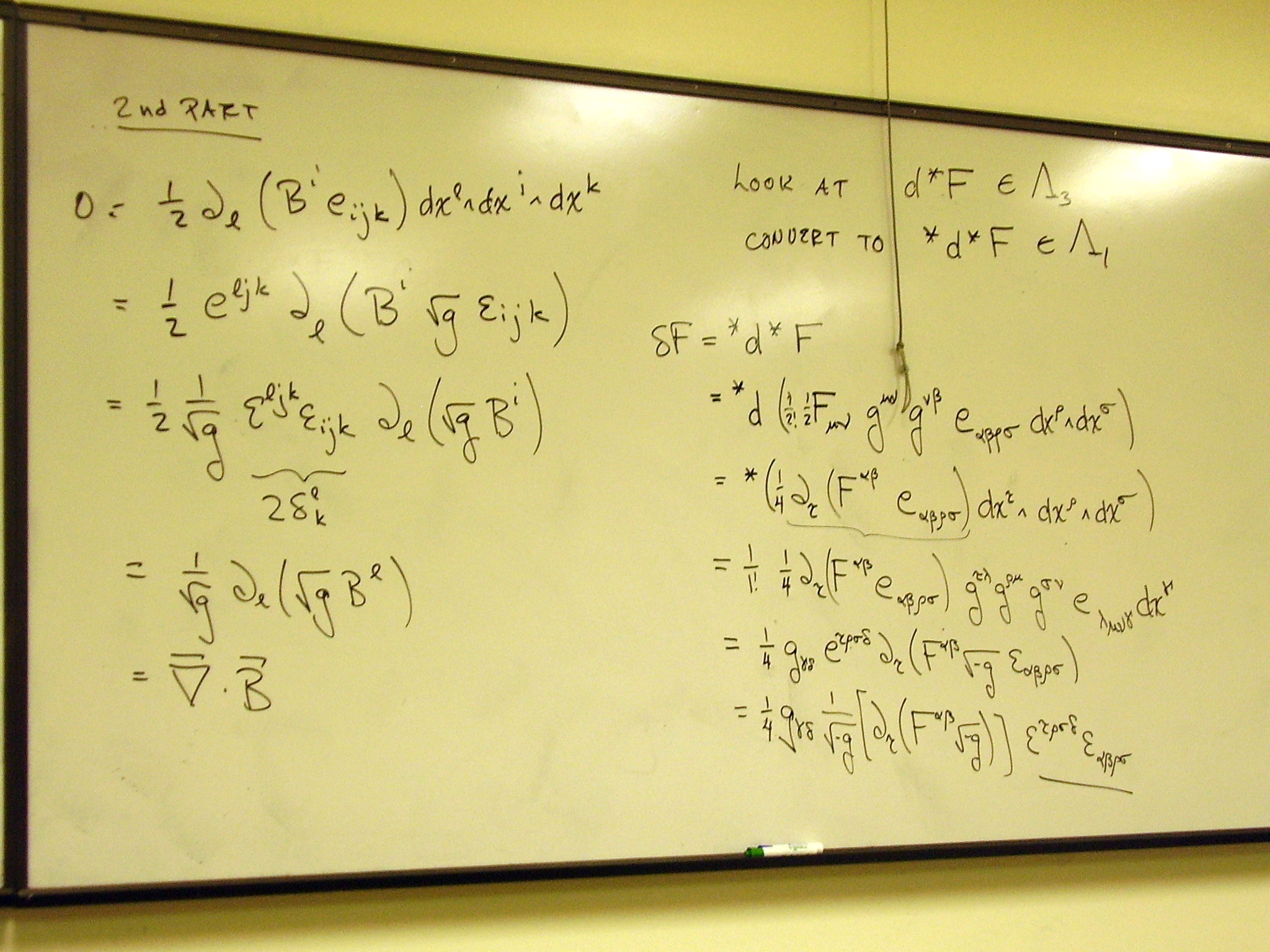
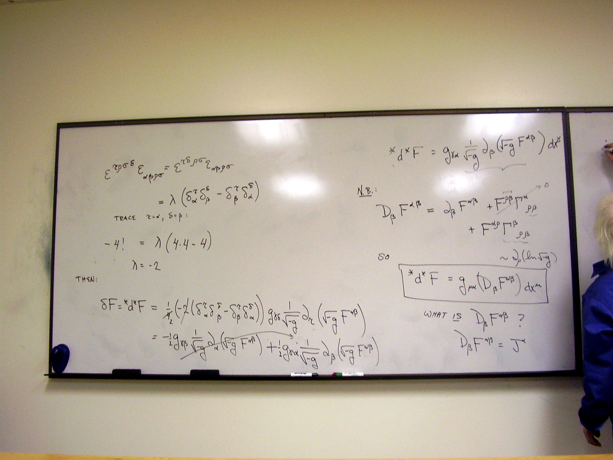
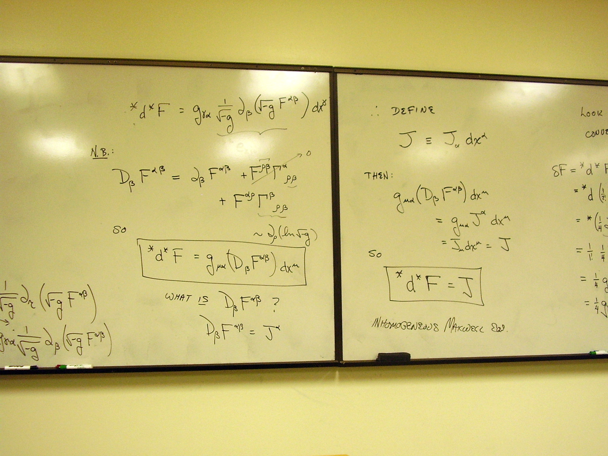
The field in terms of the
potential; the two Maxwell equations; the continuity equation. (Note that the
first and last follow from the middle two using the Poincaré lemma and its
converse).
Wednesday, January 14,
2009
Lecture:
Coordinate vs. orthonormal bases; the Laplacian; example
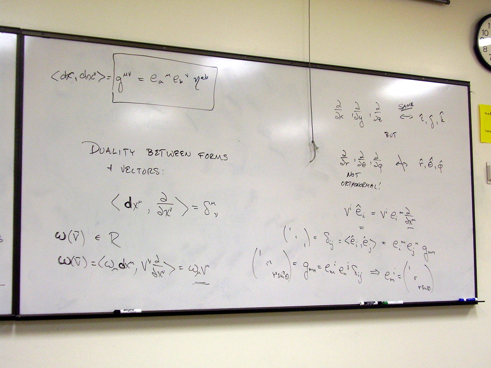
Change of basis: orthonormal
vs. coordinate bases for forms and vectors. Duality between vectors and forms.
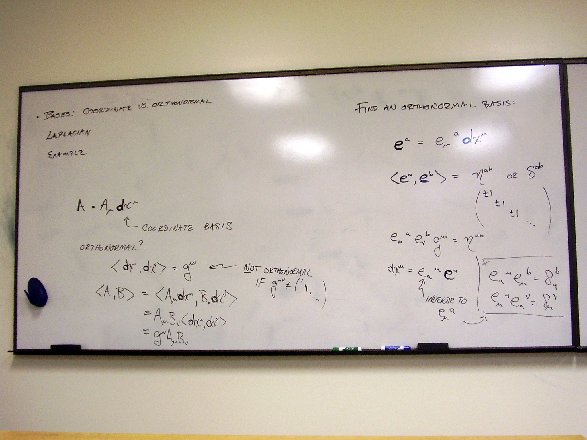
An example: finding the curl
of a vector in spherical coordinates and an orthonormal frame, starting from
the expression in differential forms.
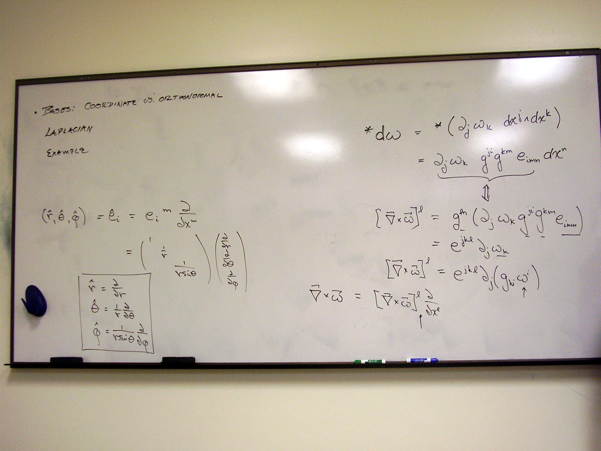
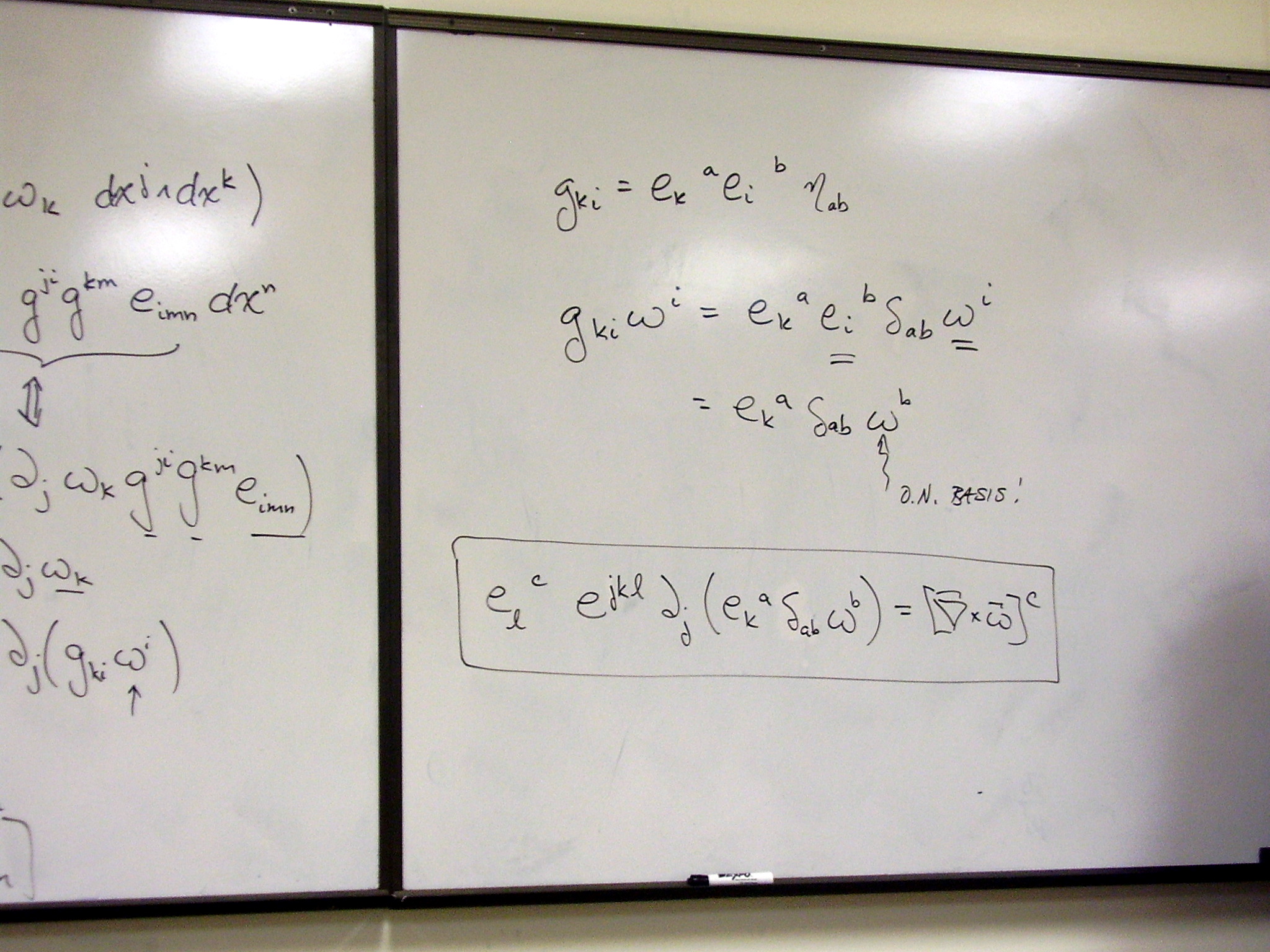
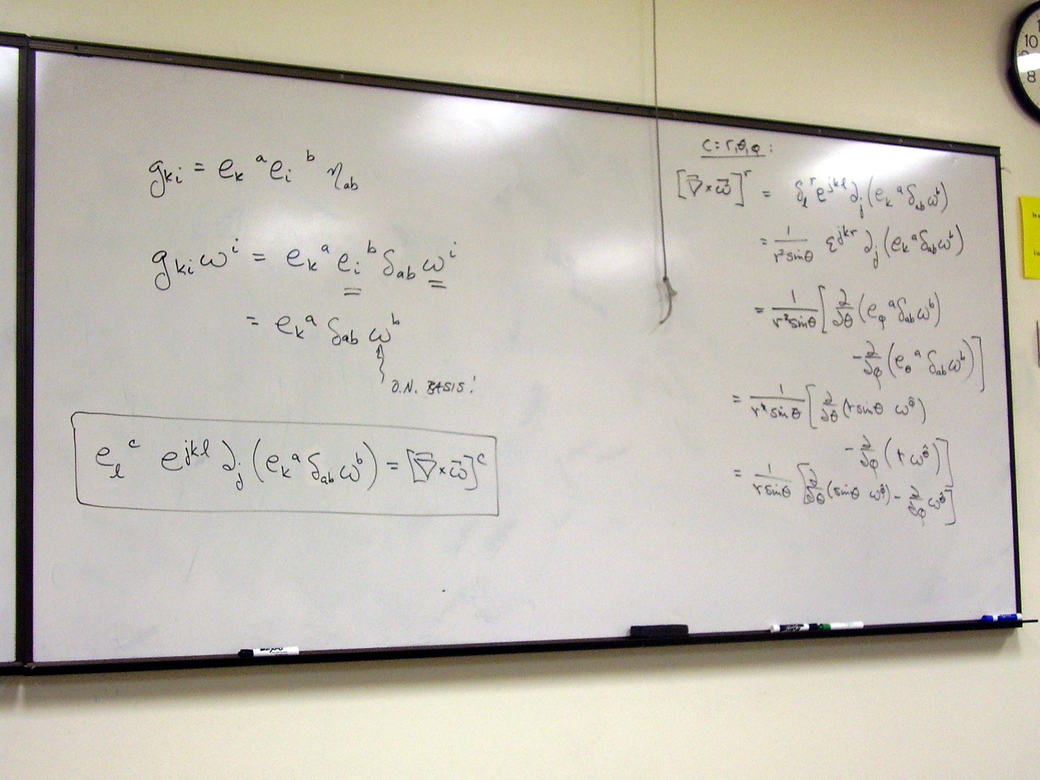
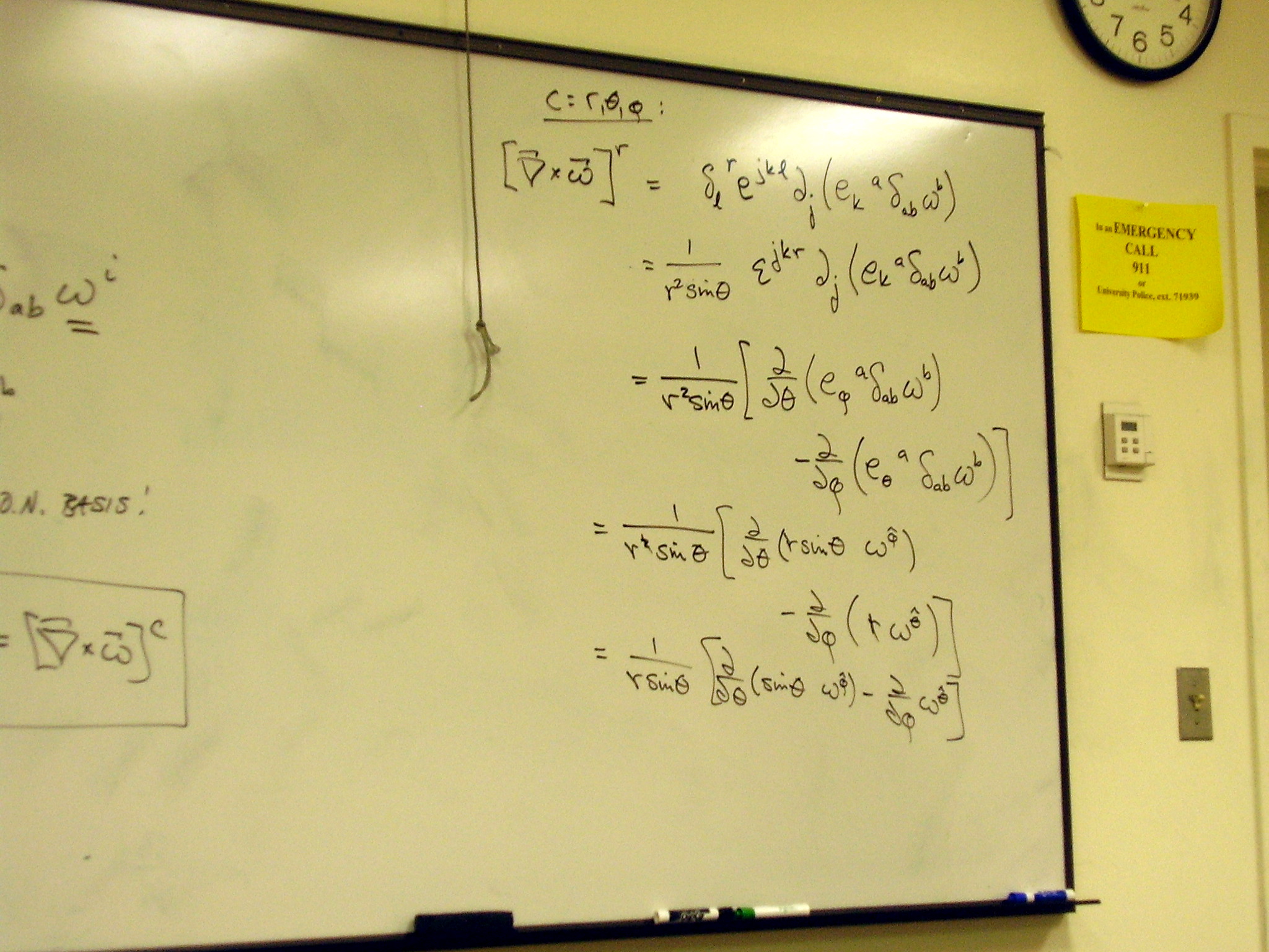
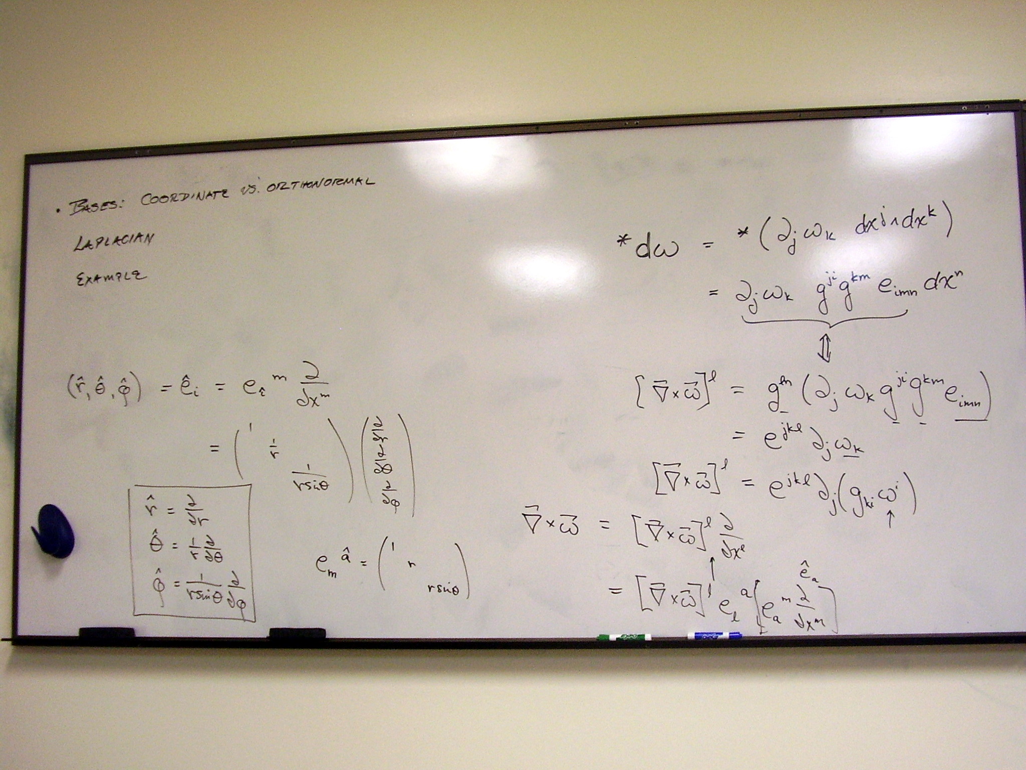
The Laplacian must be
constructed from two possible expressions:
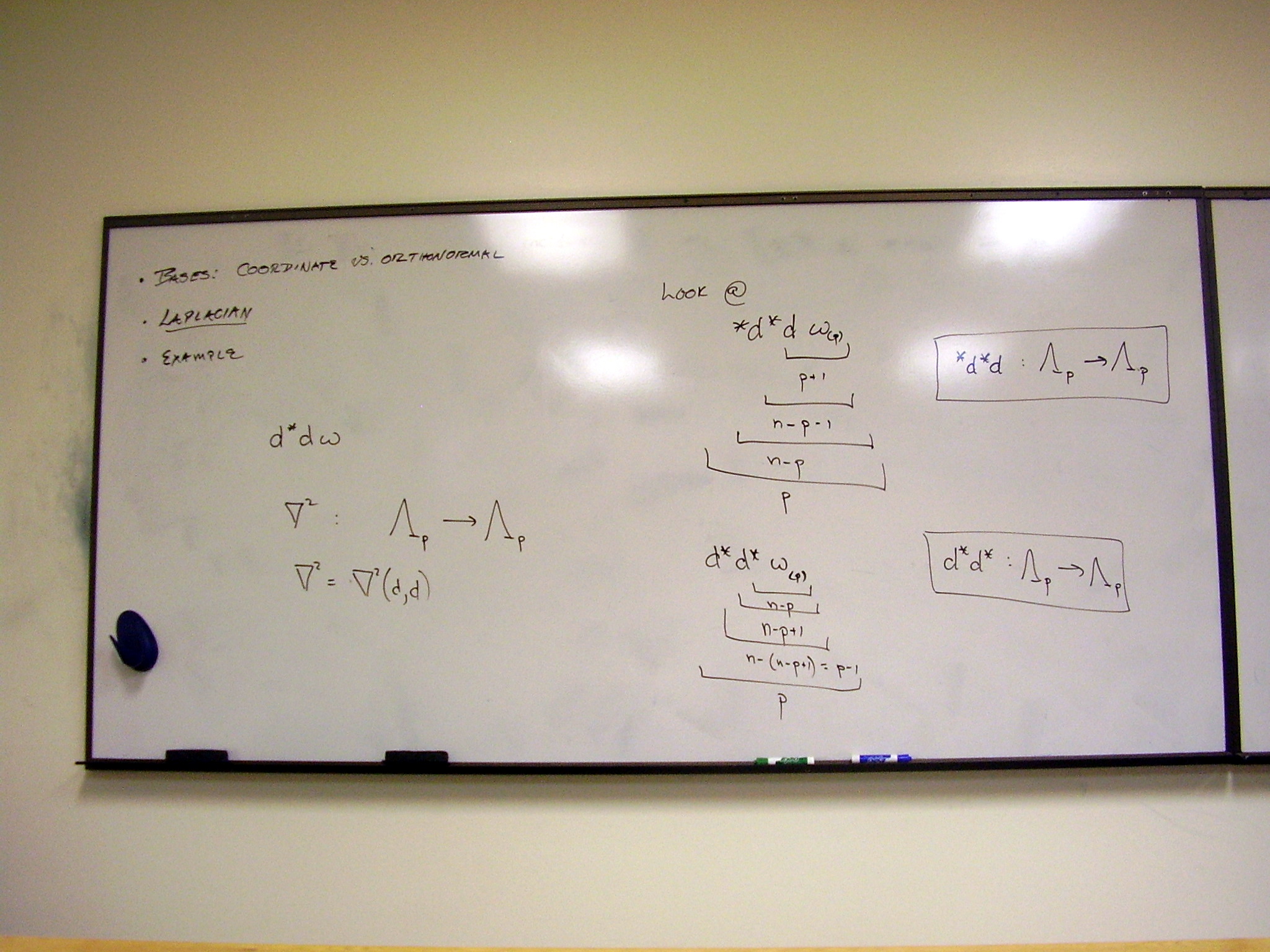
The Laplacian of a function:
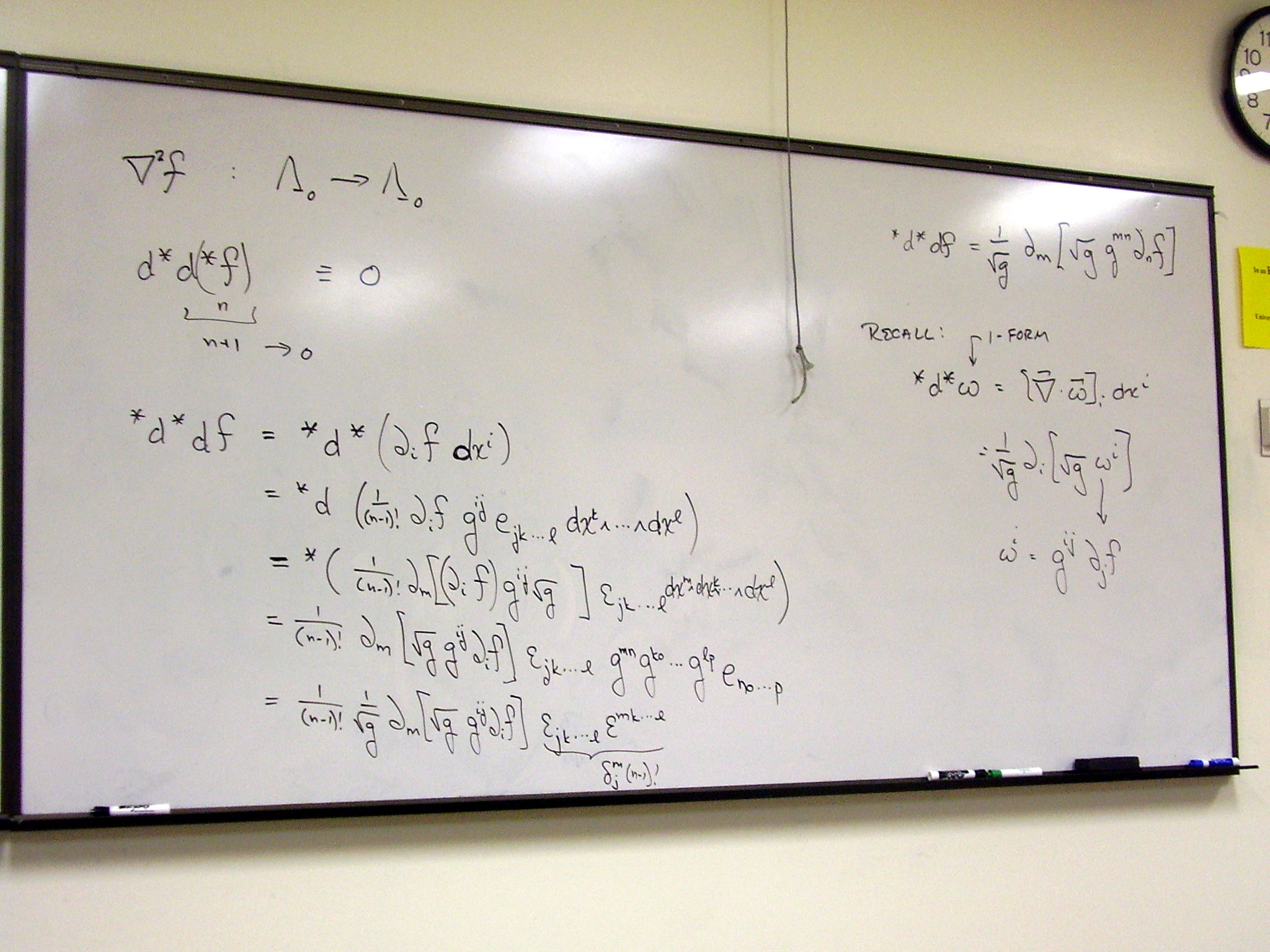
The Laplacian of a 1-form:
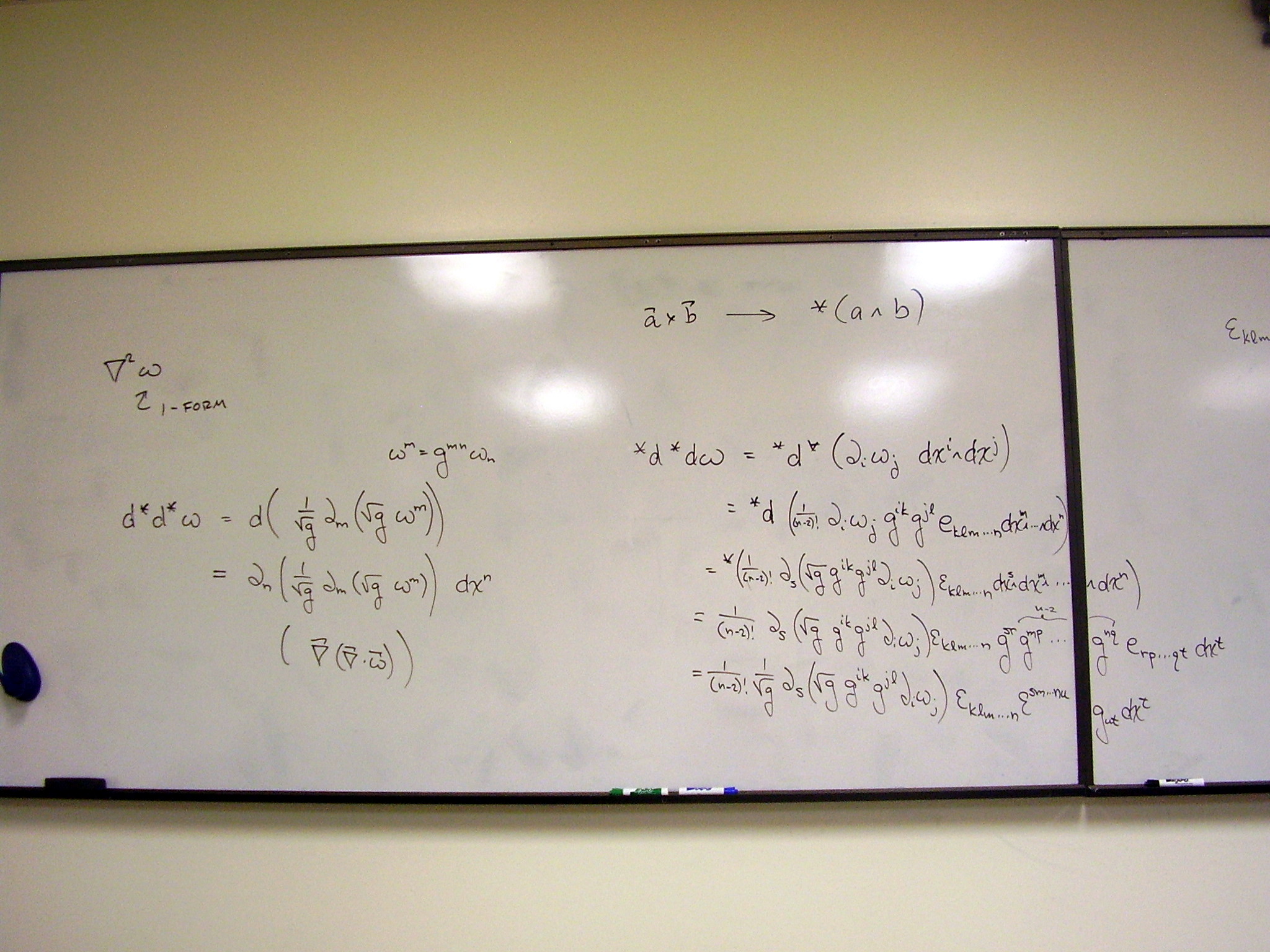
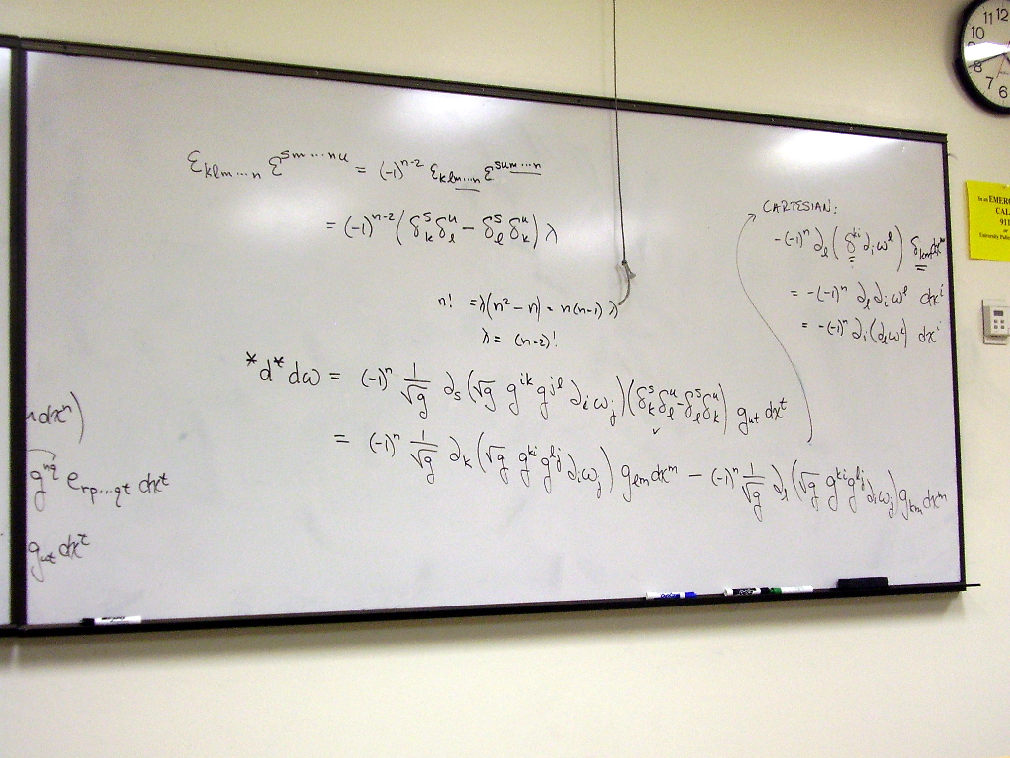
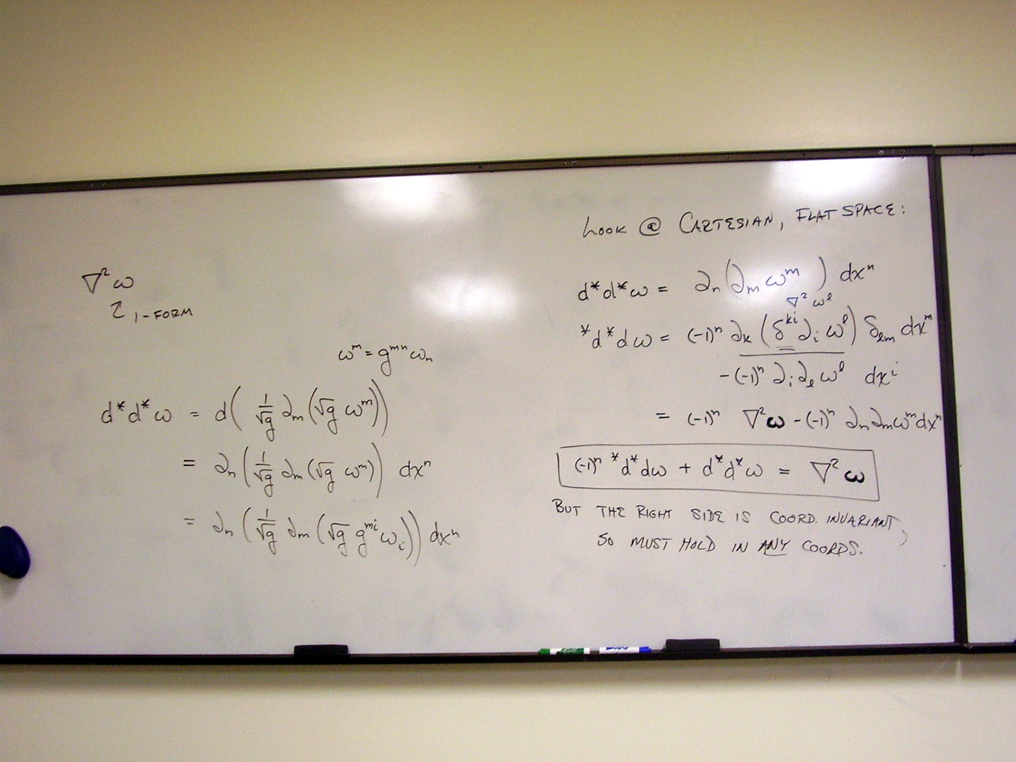
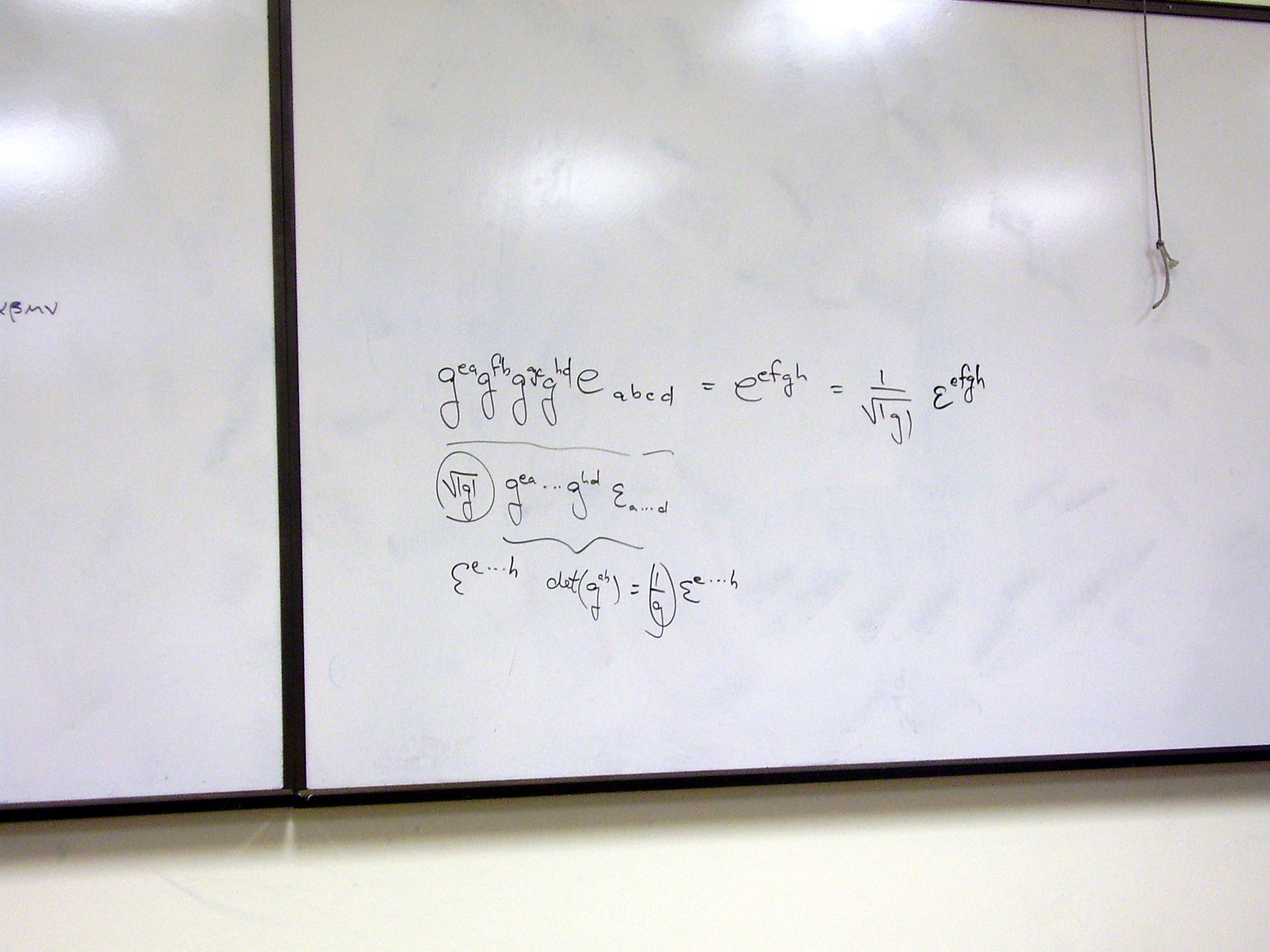
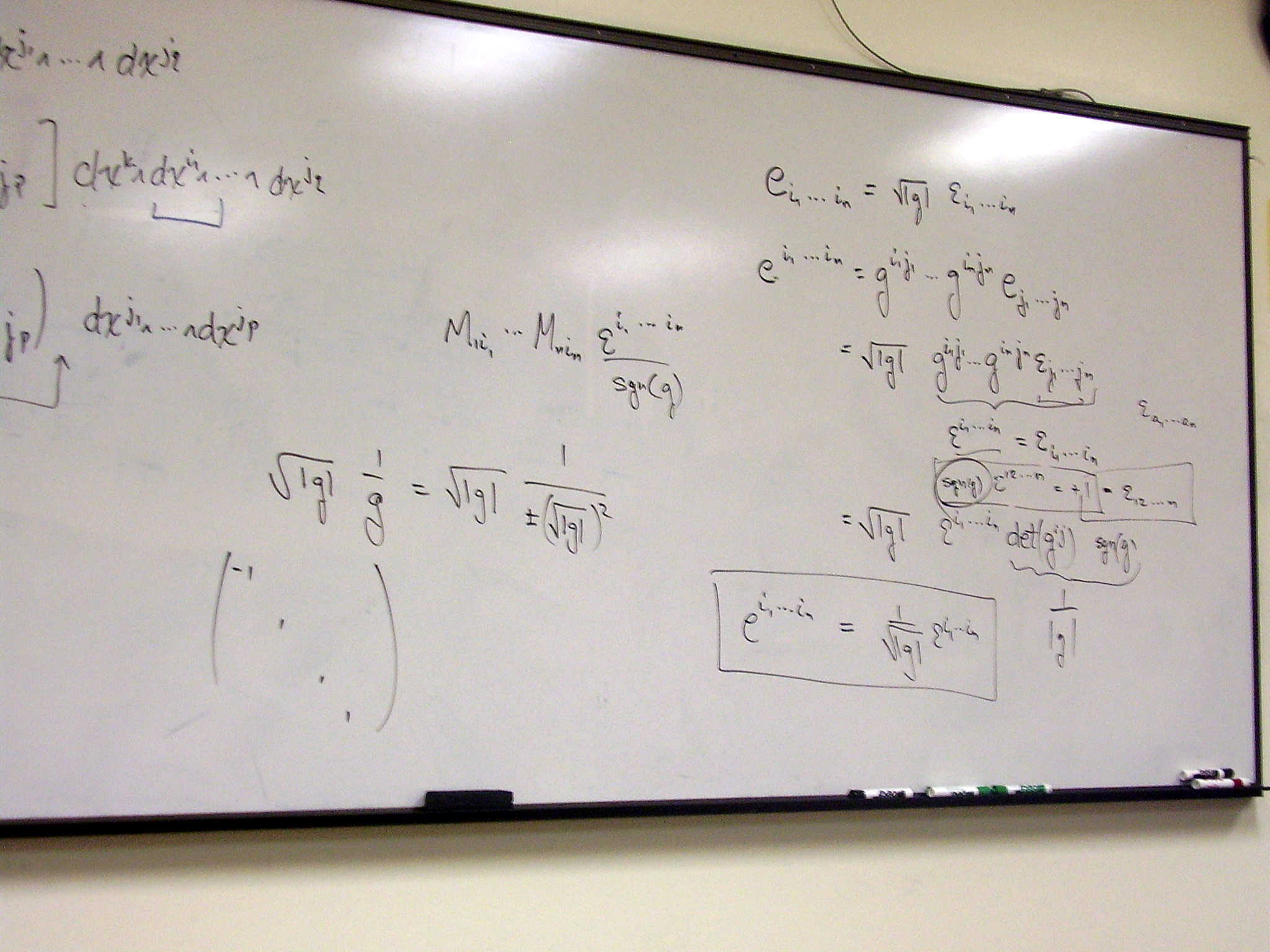
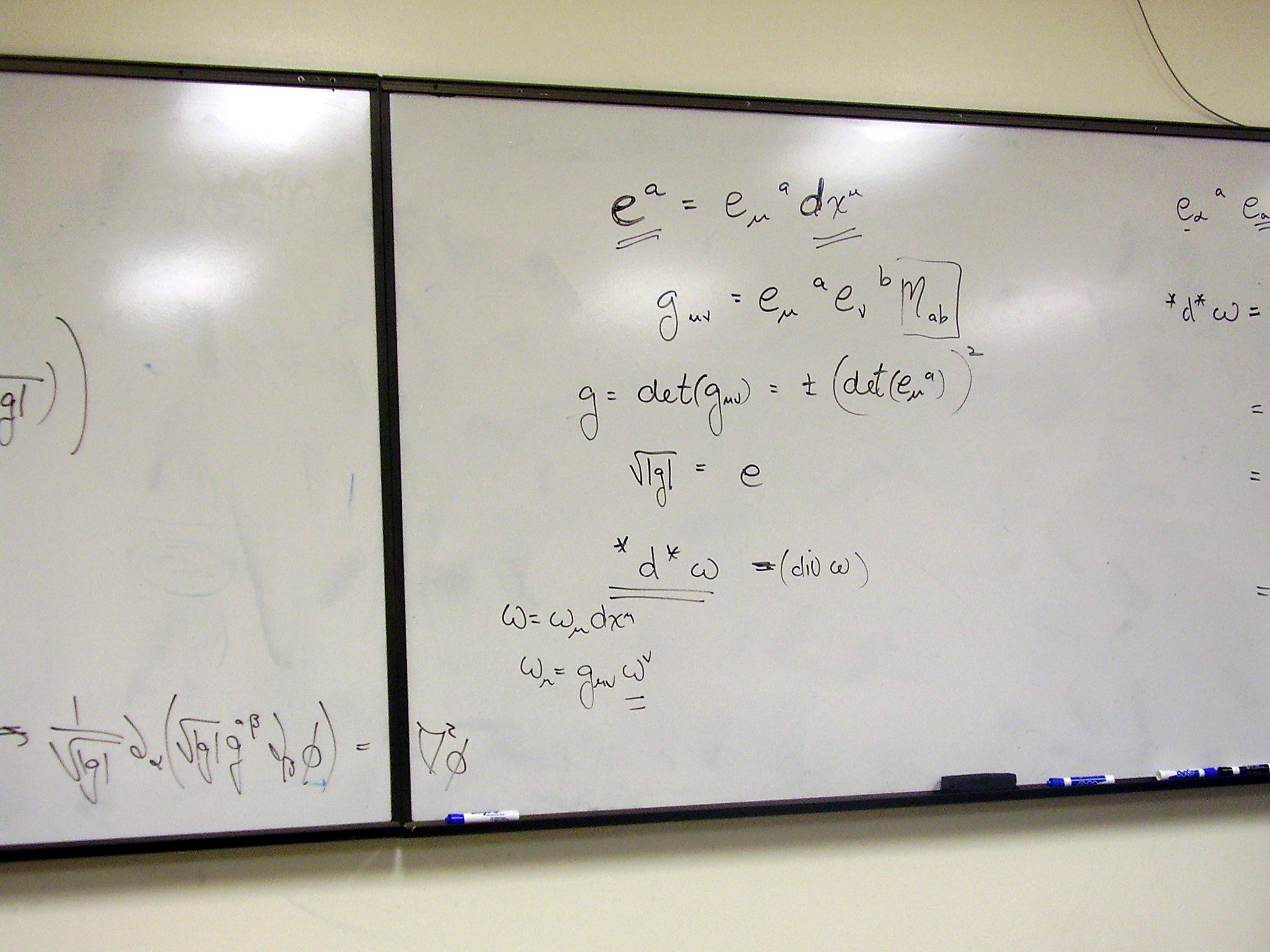
Checking the components of
the dual of the Maxwell field tensor; checking the sign of the contravariant
Levi-Civita tensor:
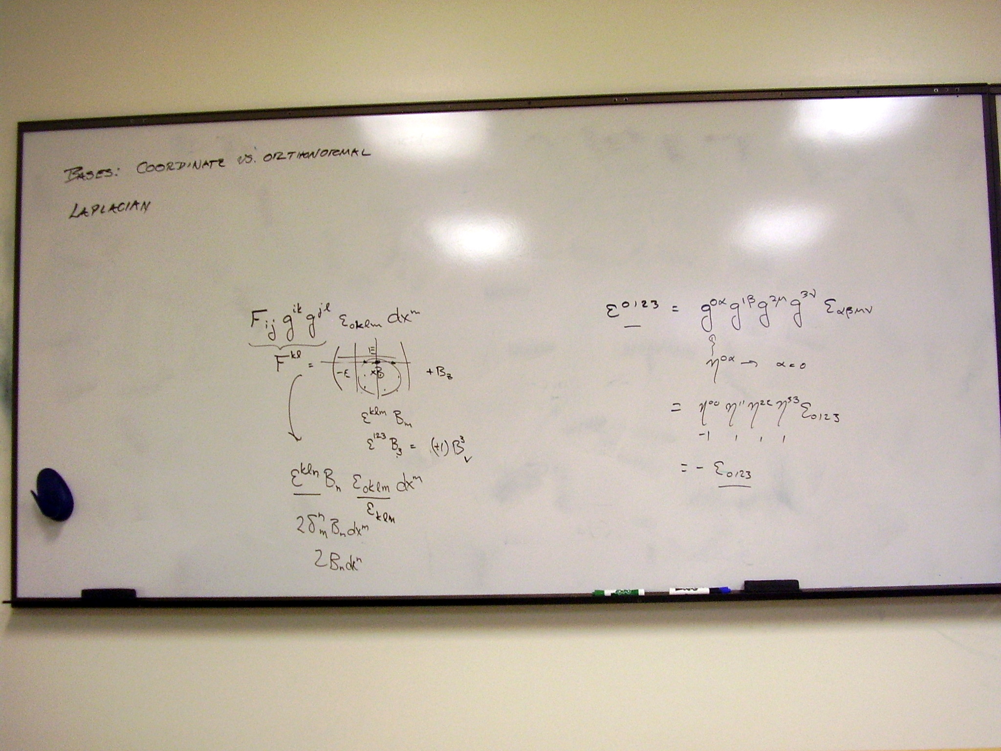
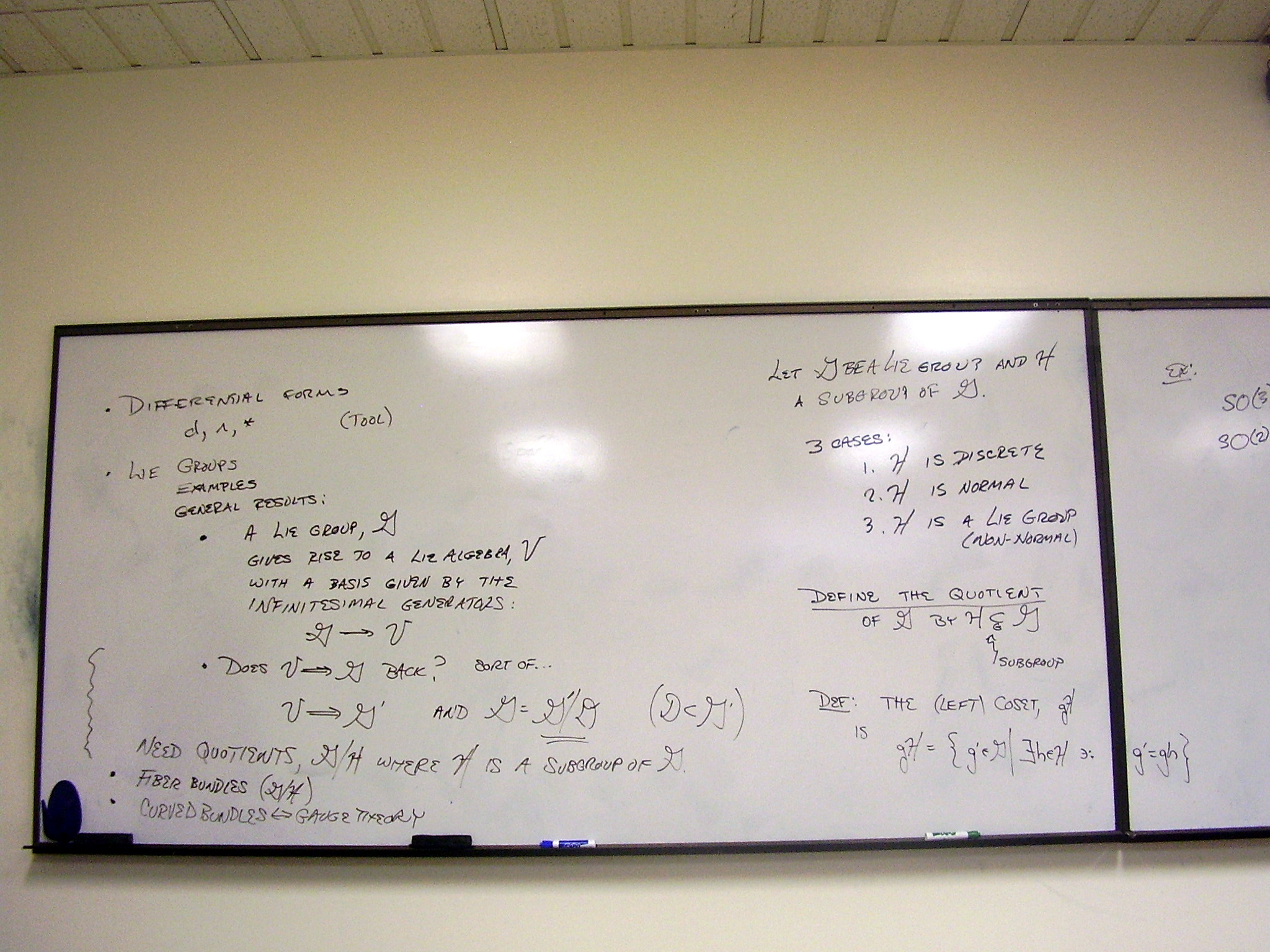
B. Lie
groups and Lie algebras
Friday, January 16,
2009
Lecture:
Group theory; finite groups
Translating between vector
formulas and exterior calculus – a dictionary:
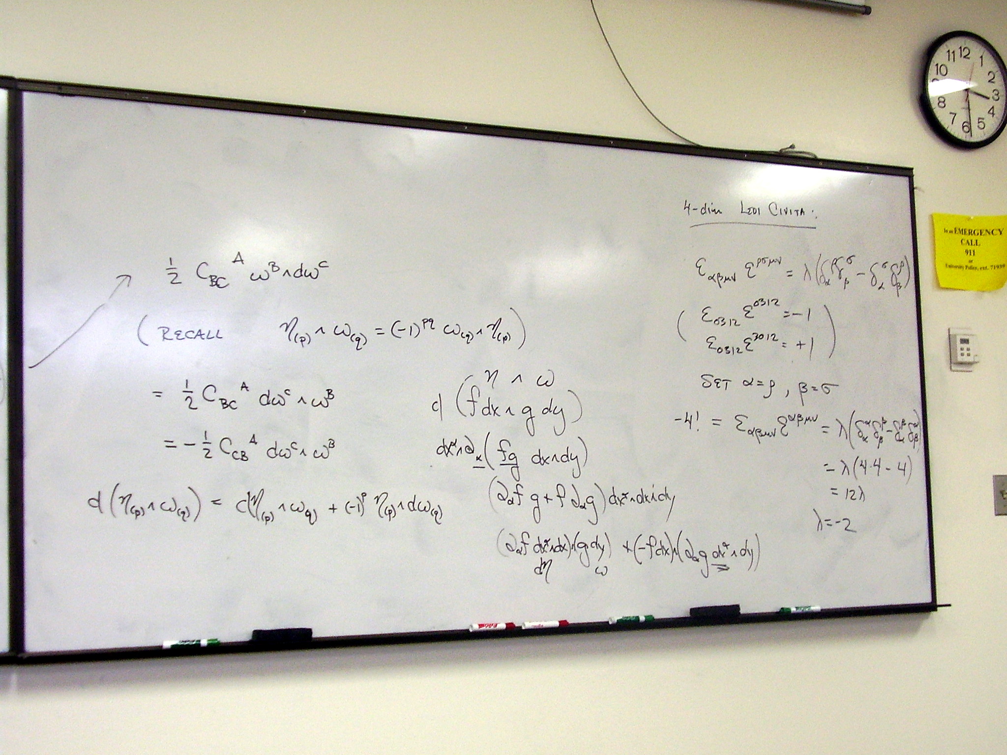
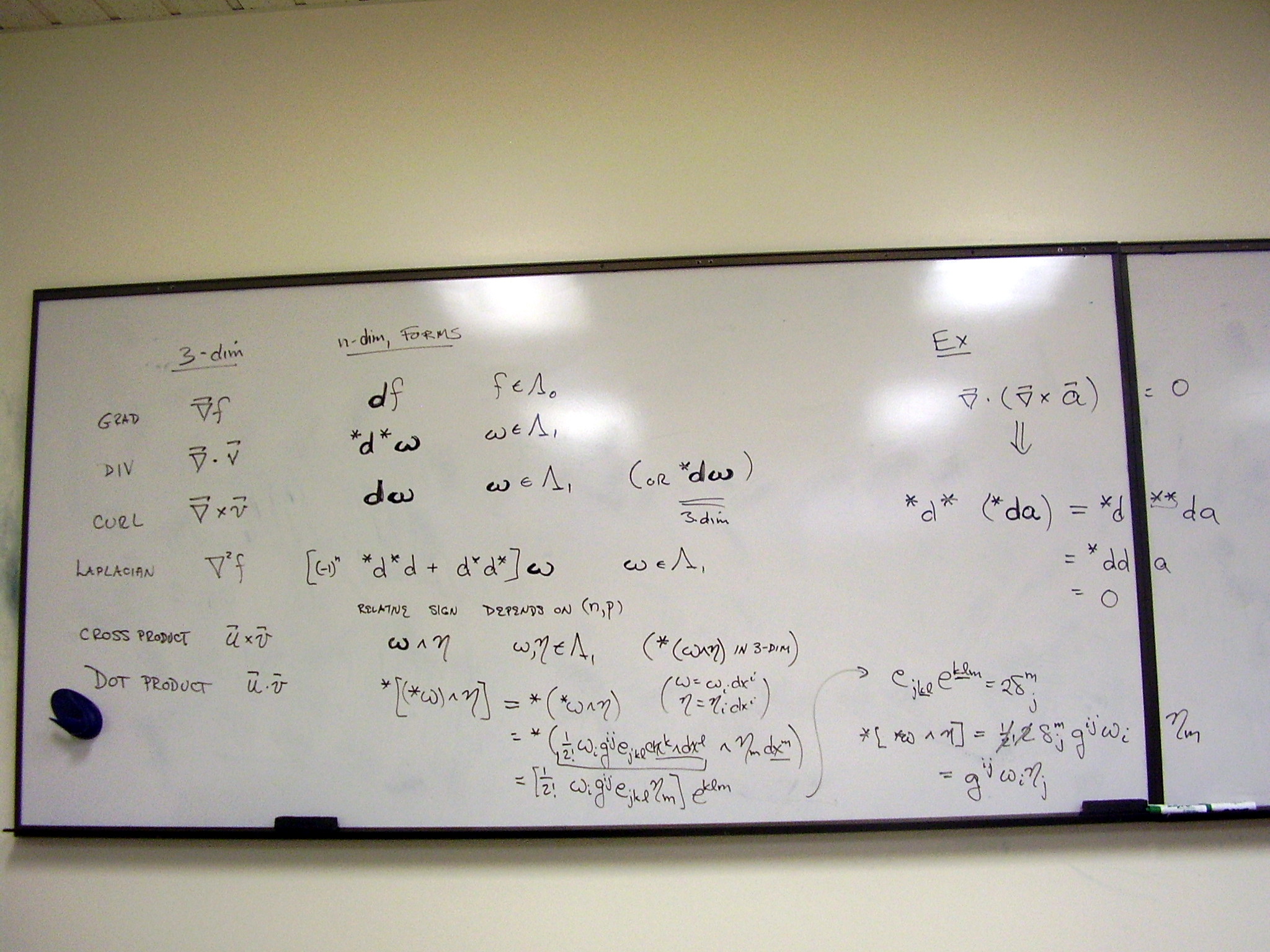
The Levi-Civita tensor
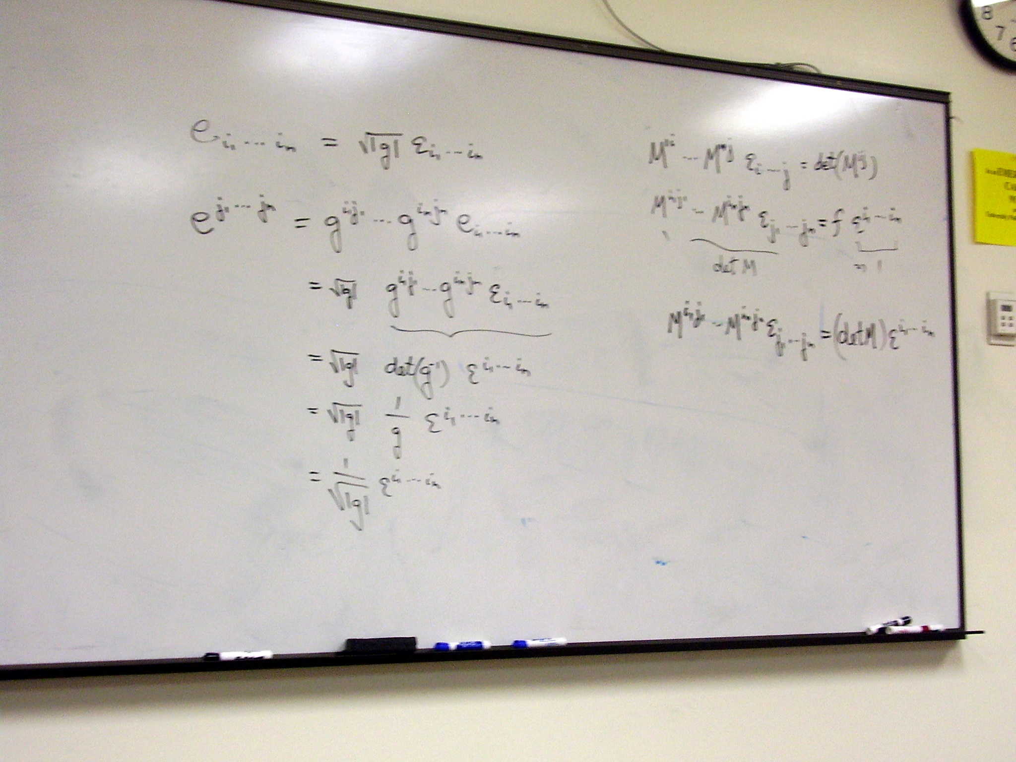
Definition of a group:
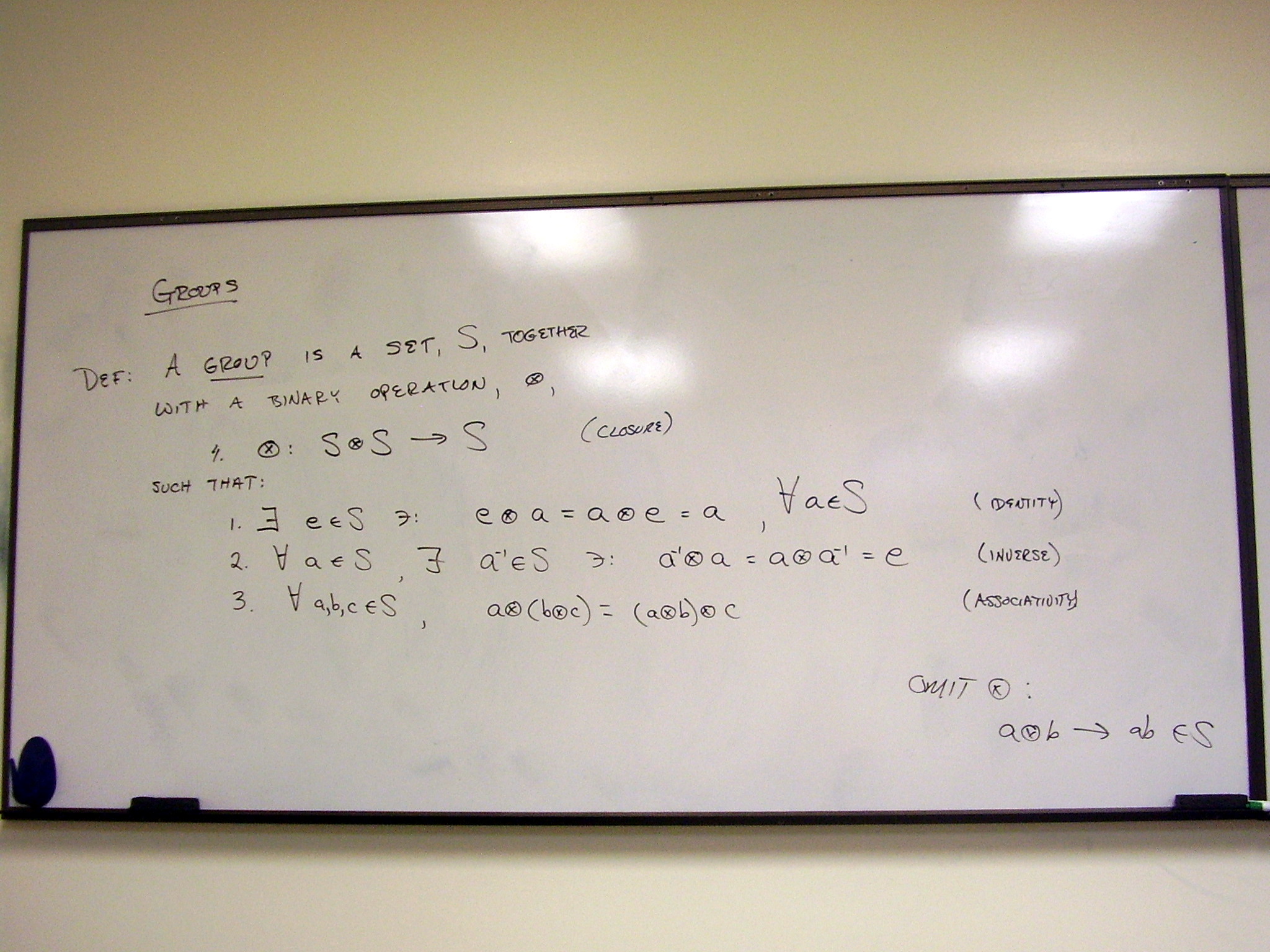
Simple examples of groups:
one, two and three element groups.
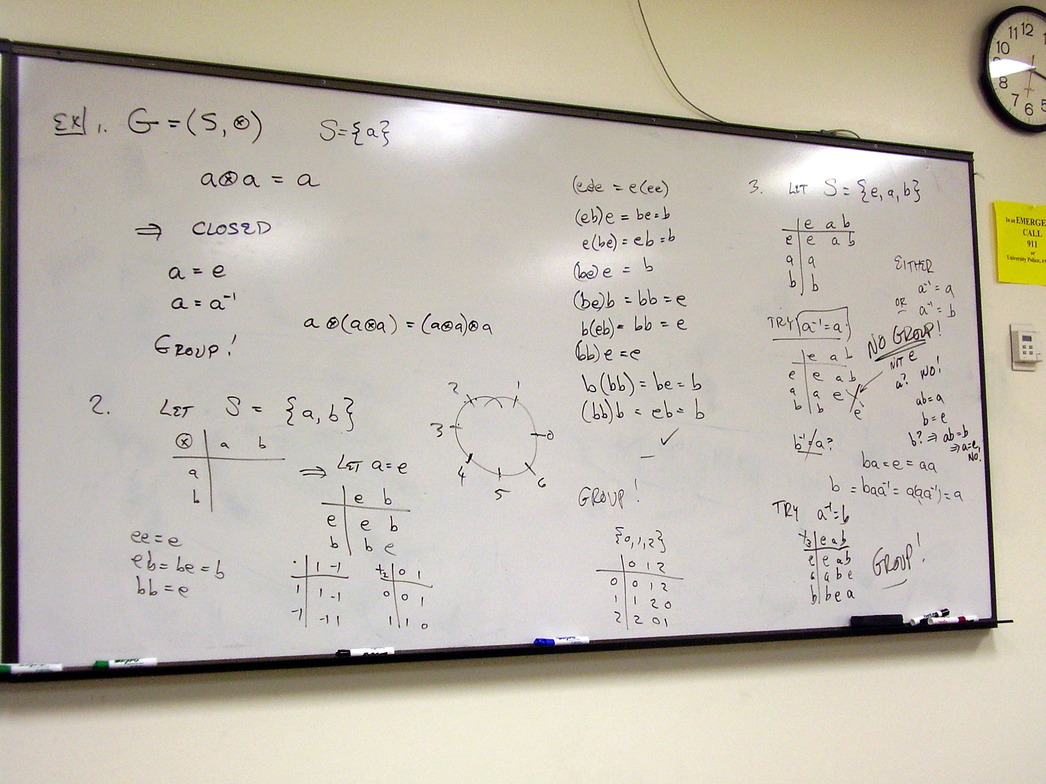
A general result, and two
4-element groups:
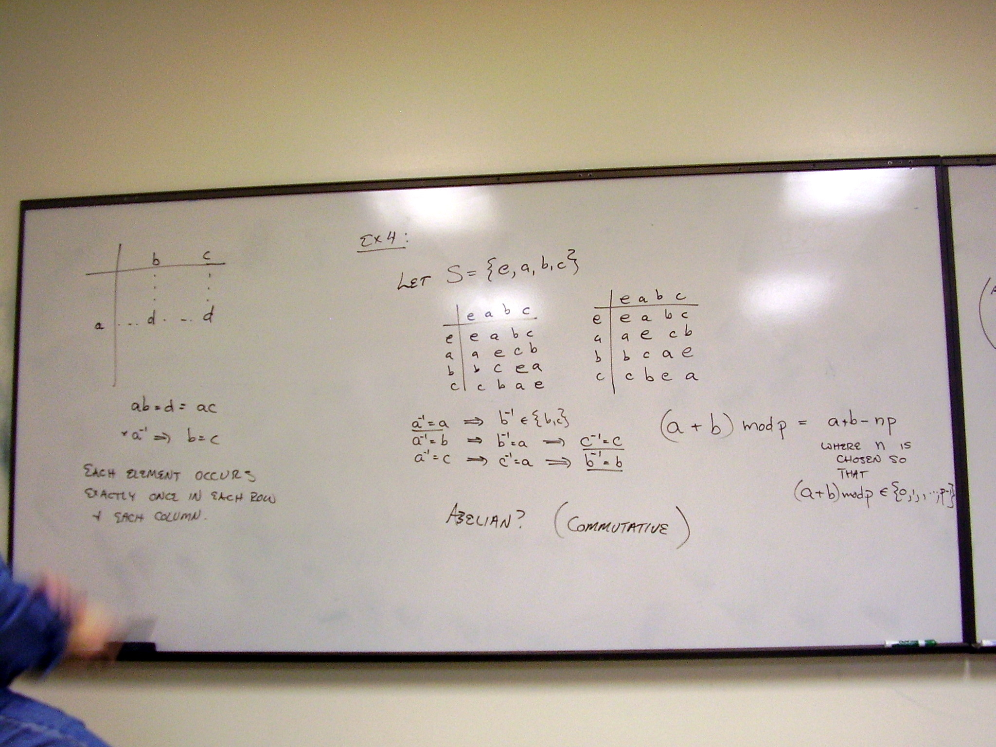
5-elements; product
groups; is the 6-element cyclic group a product group?
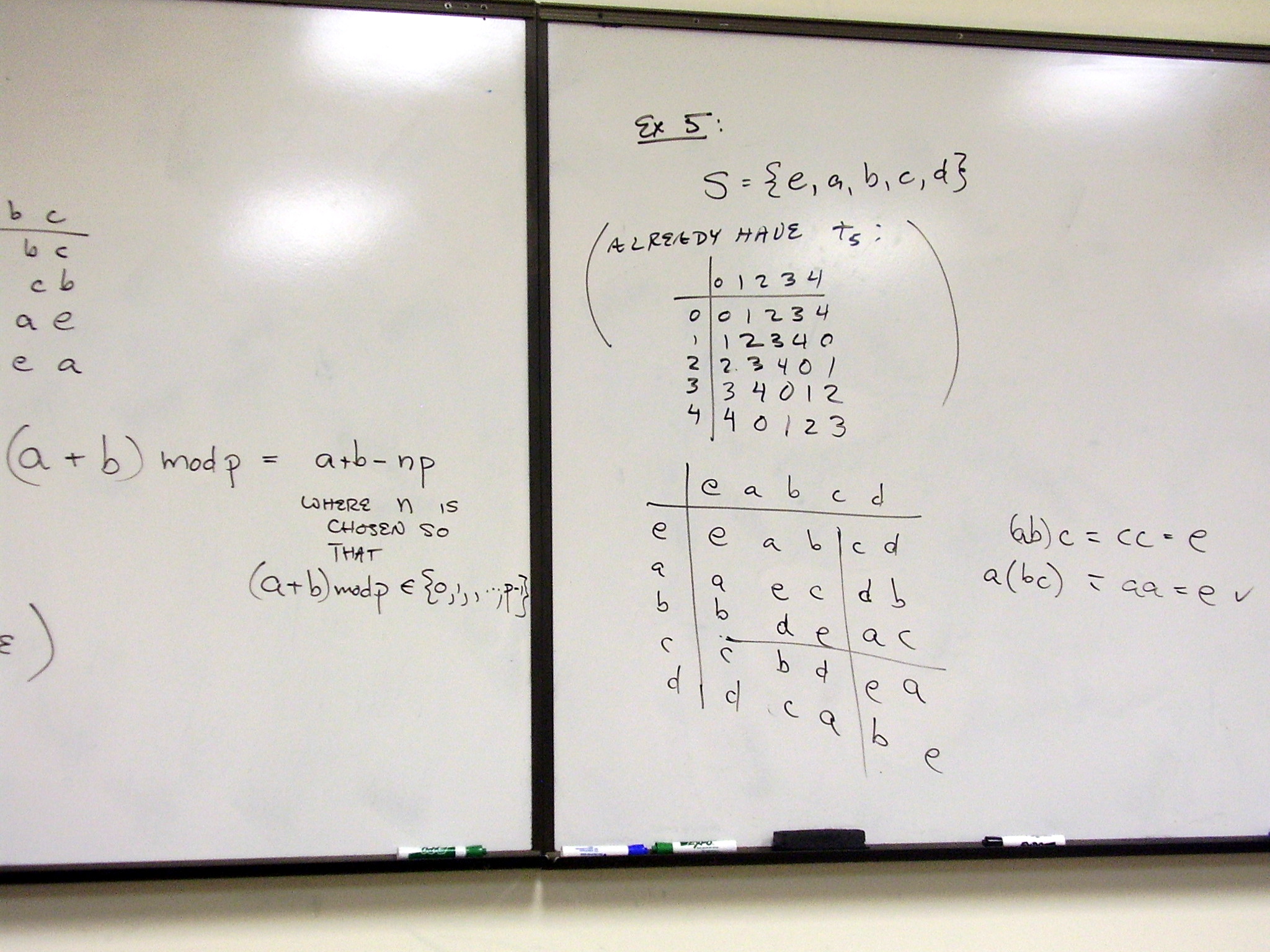
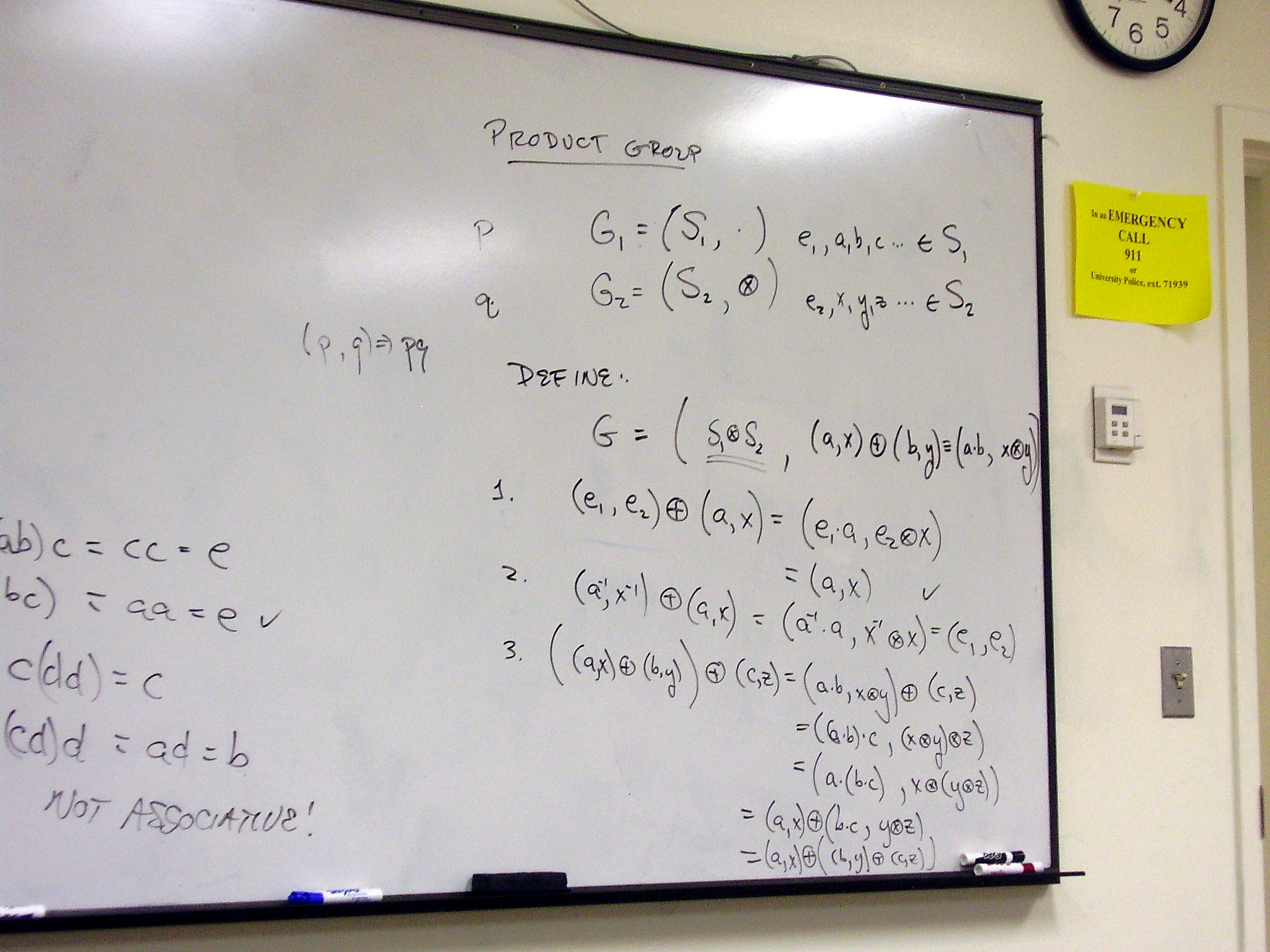
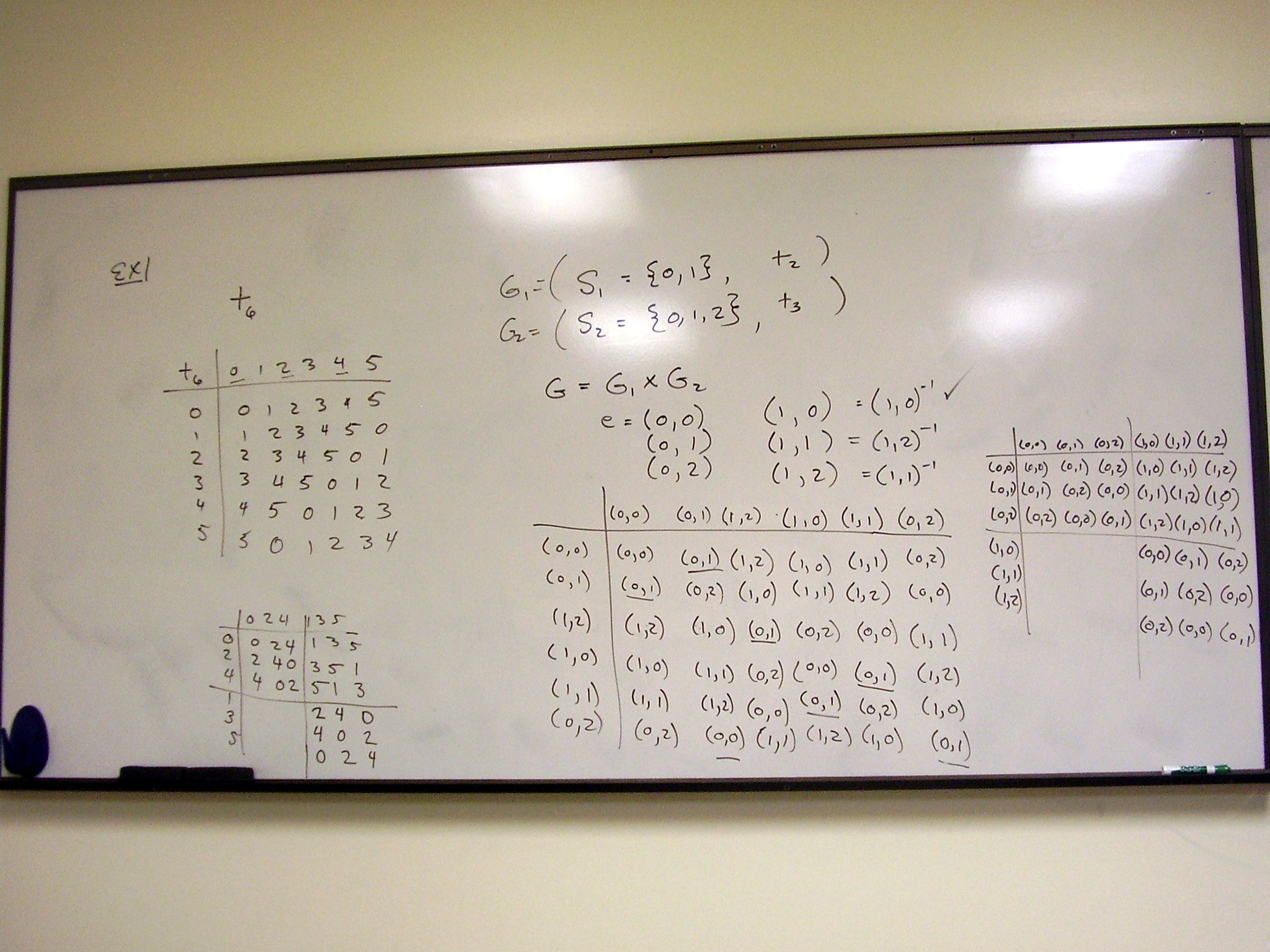
Wednesday, January 21,
2009
Lecture:
Group theory: Lie groups
A few comments on
differential forms:
The exterior derivative of
the wedge product of a p-form with a q-form:
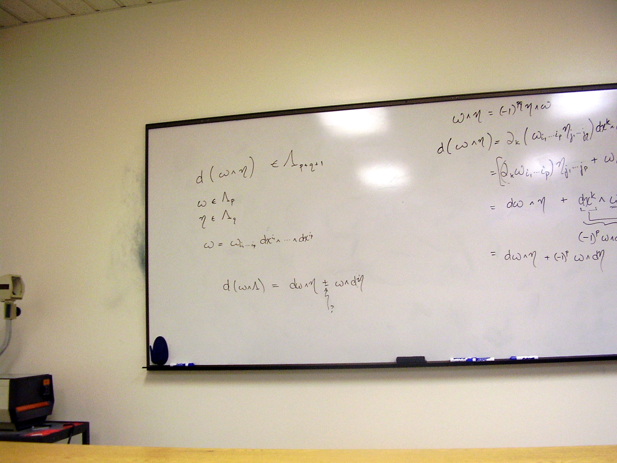
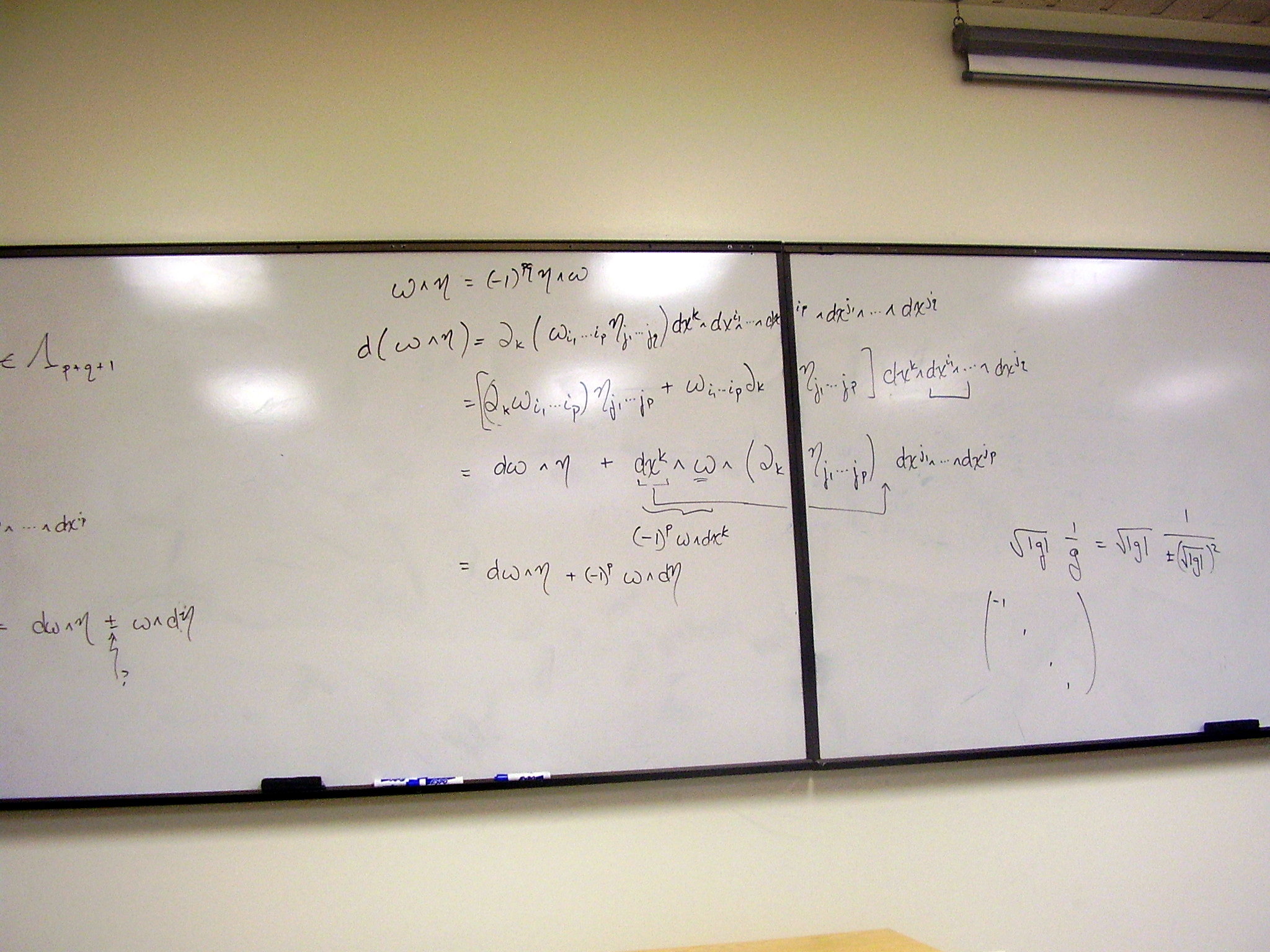
Details of the form of the
Levi-Civita tensor
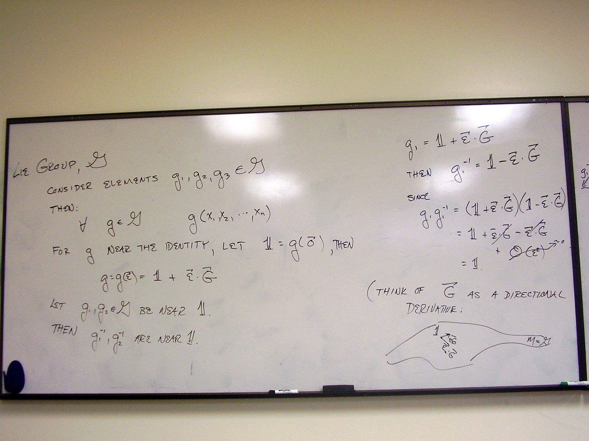
The definition of a Lie
group: (start of example)
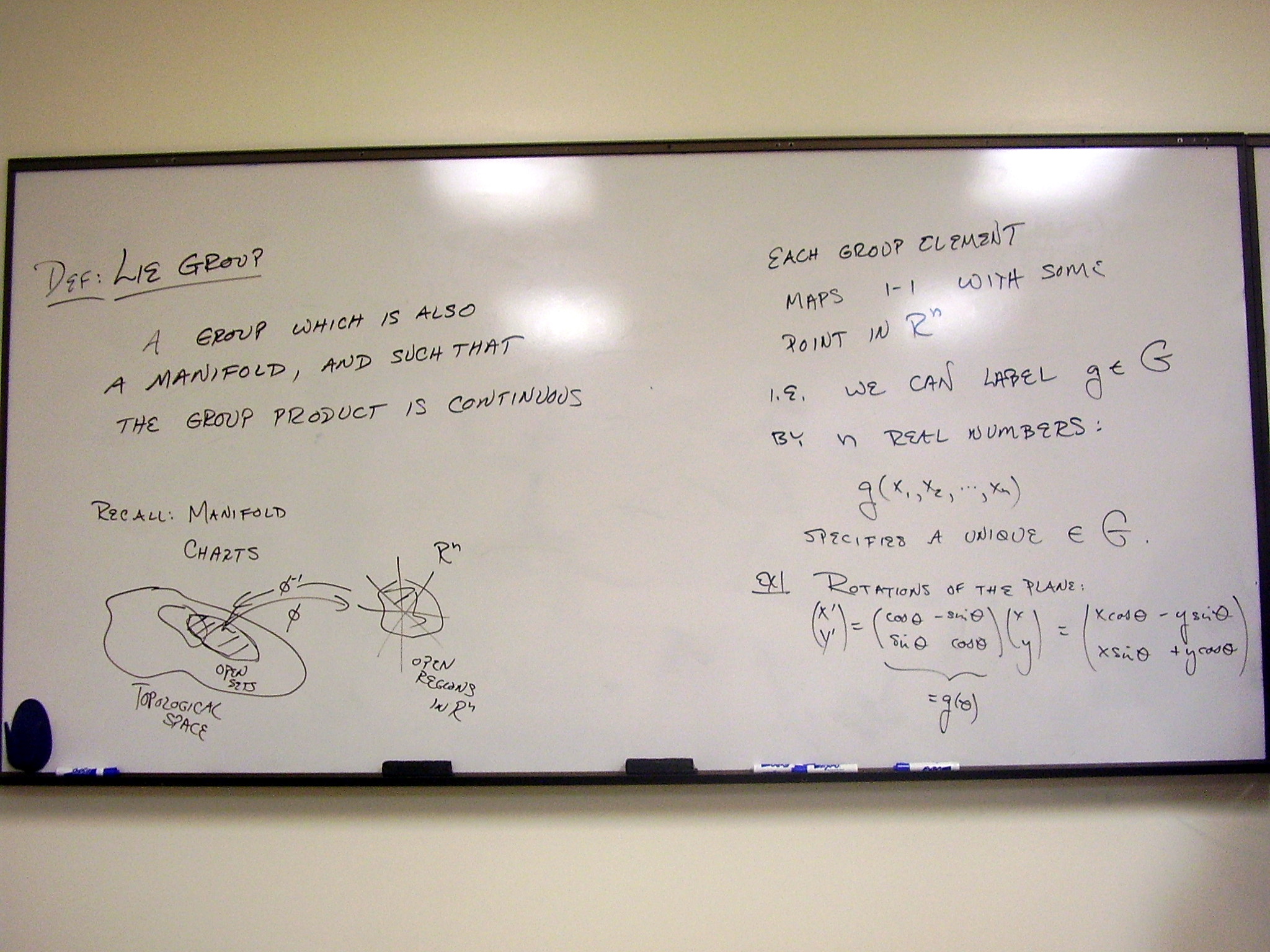
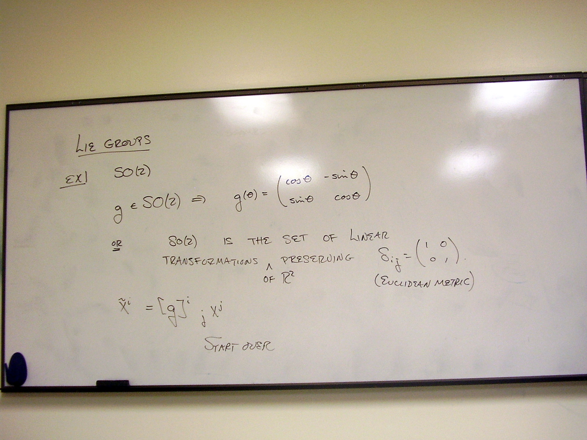
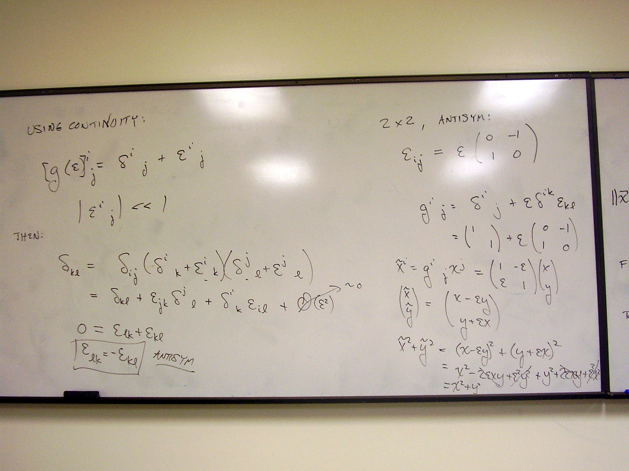
An example in detail
– rotations in the plane:
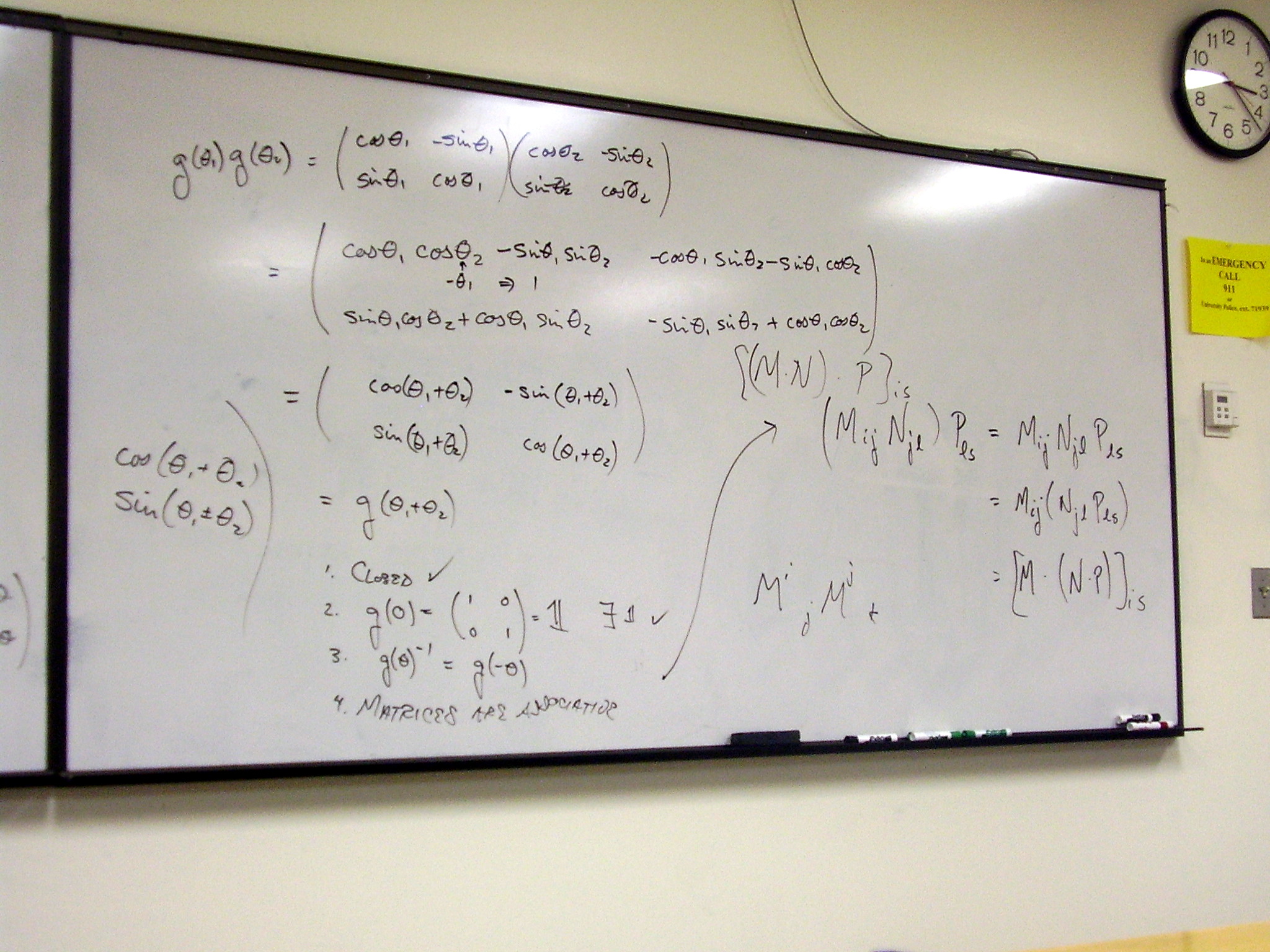
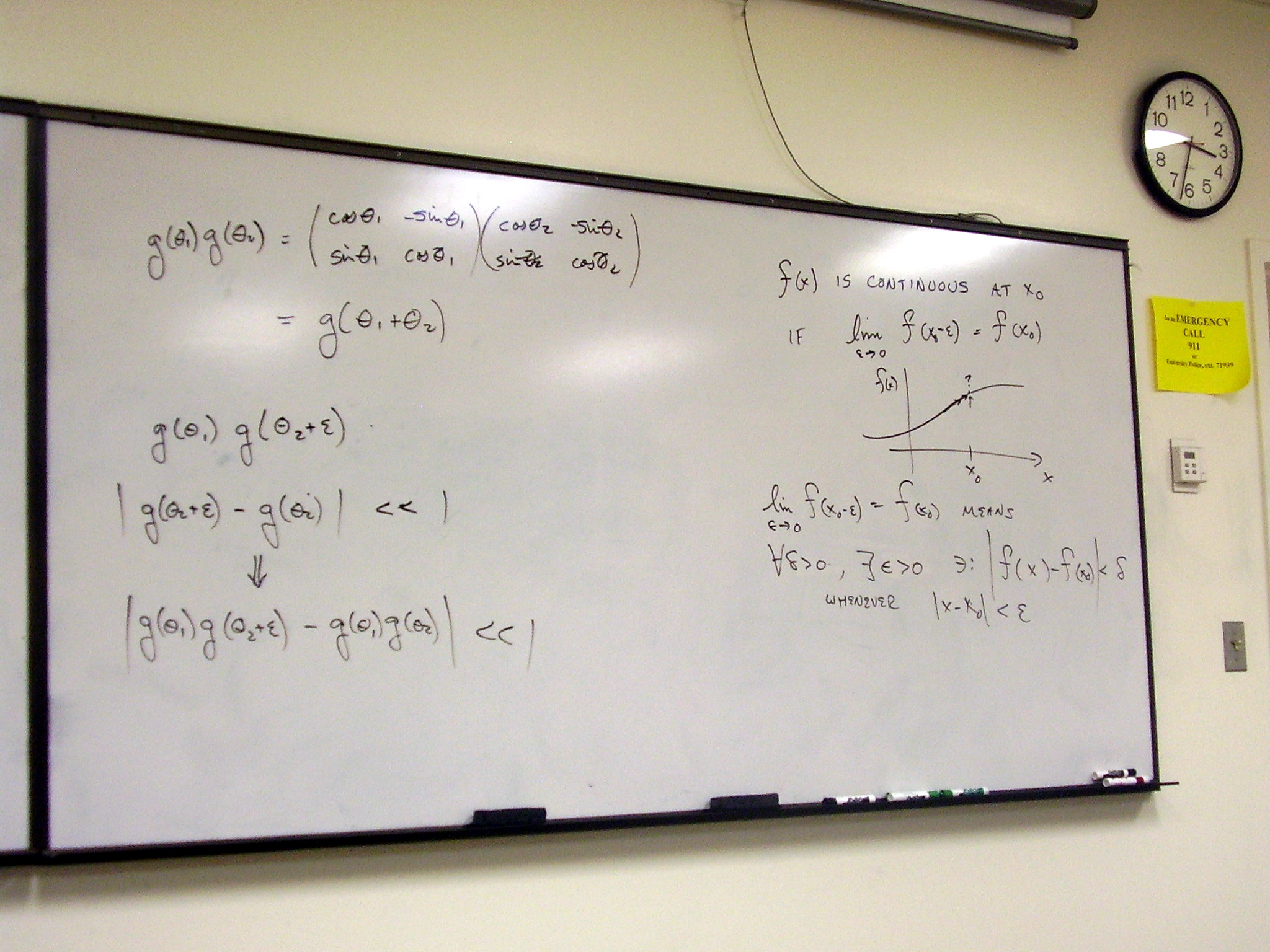
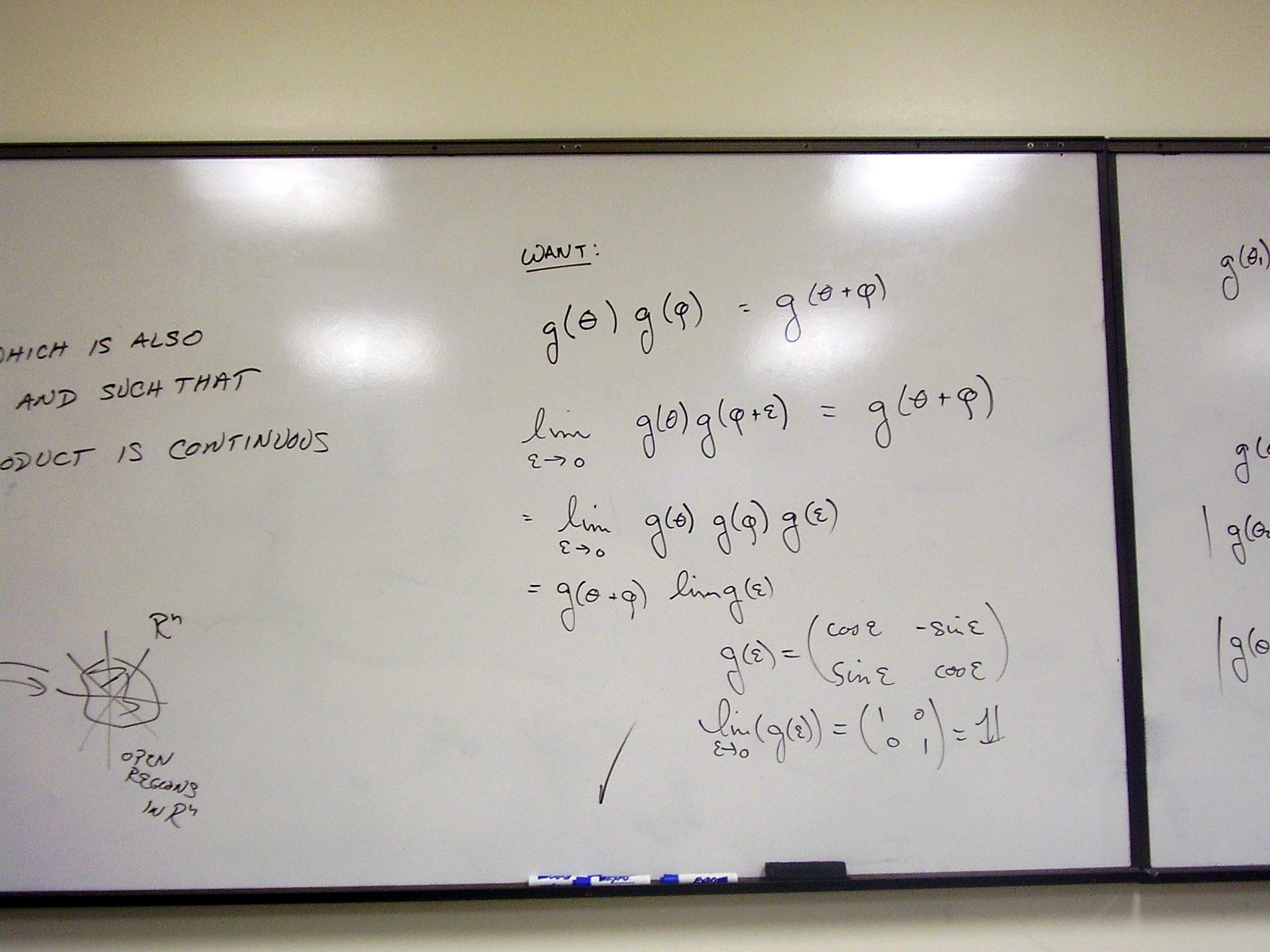
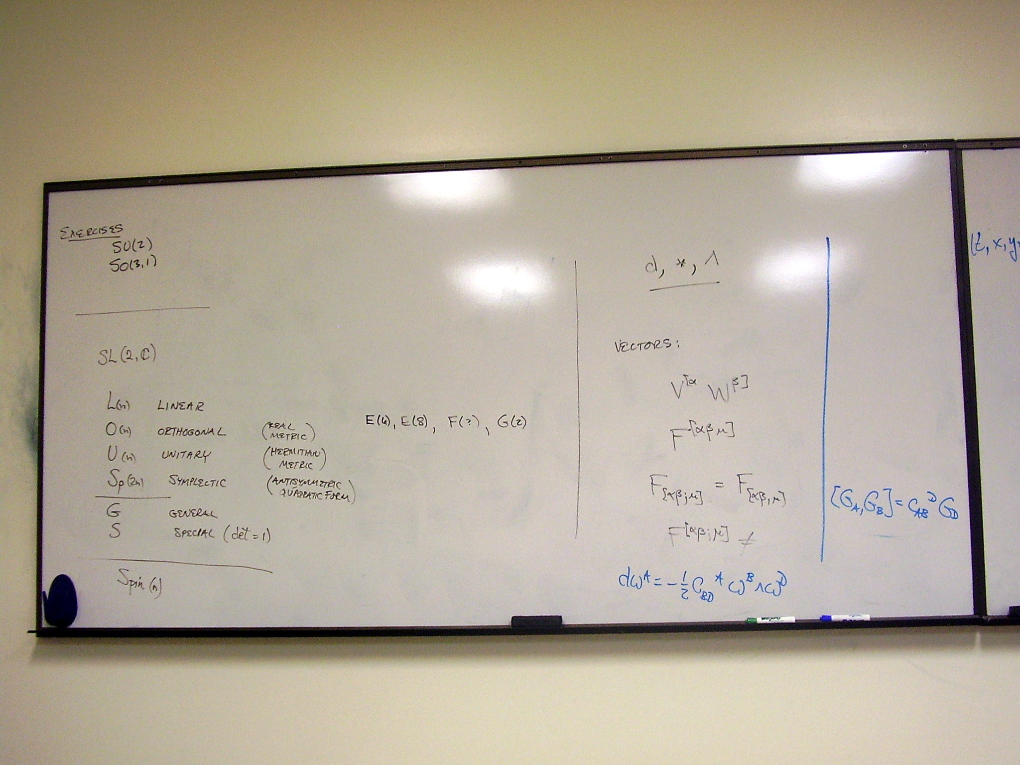
Some group nomenclature.
Further examples.
Orthogonal, O(n), and
special orthogonal, SO(n), groups:
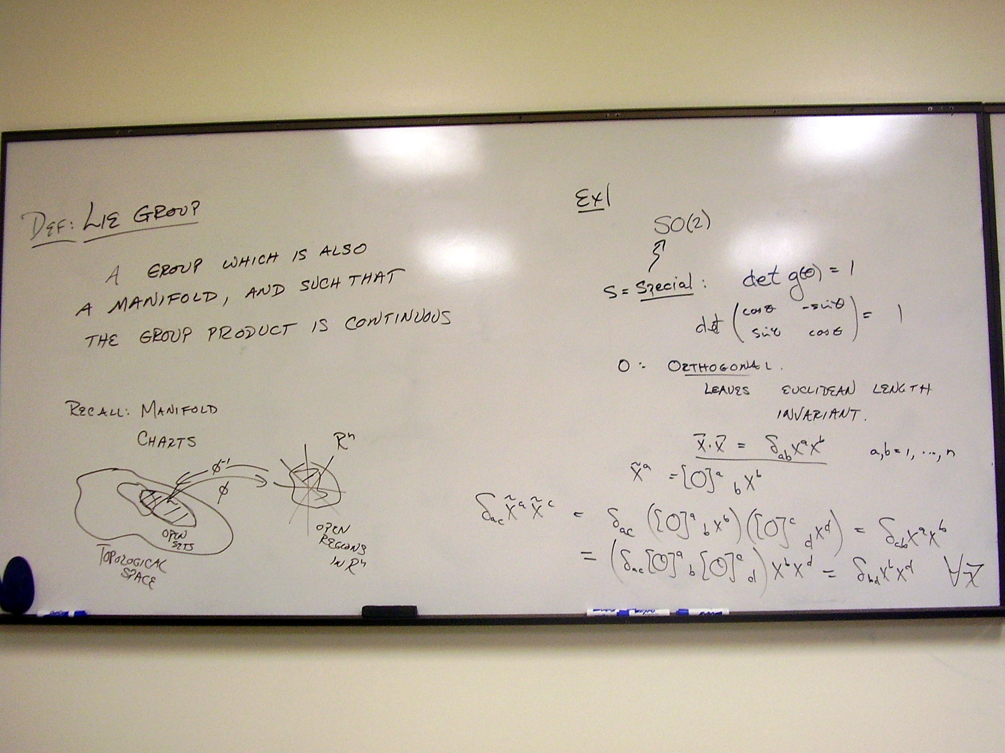
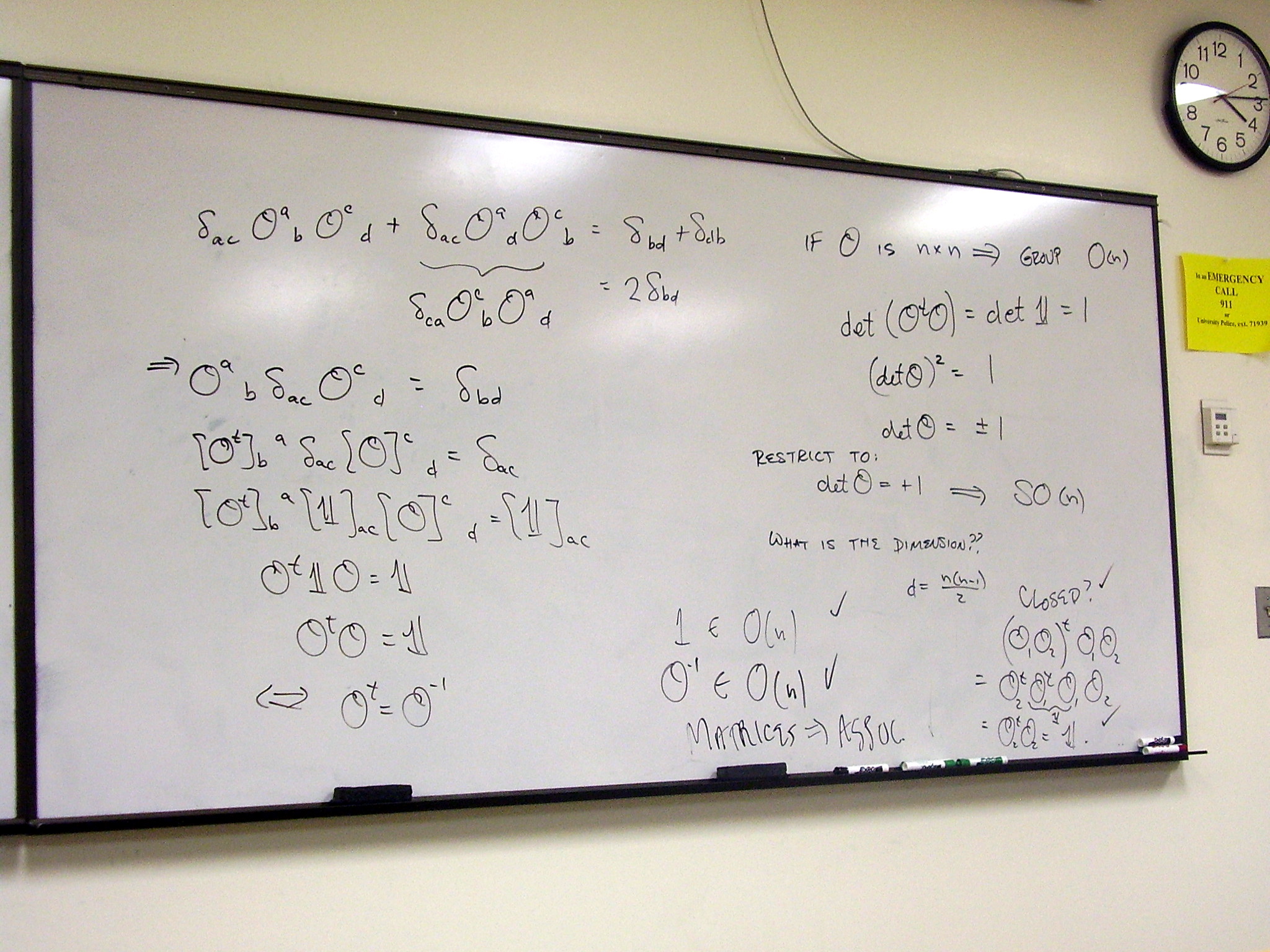
General linear, GL(n), and
special linear, SL(n), groups
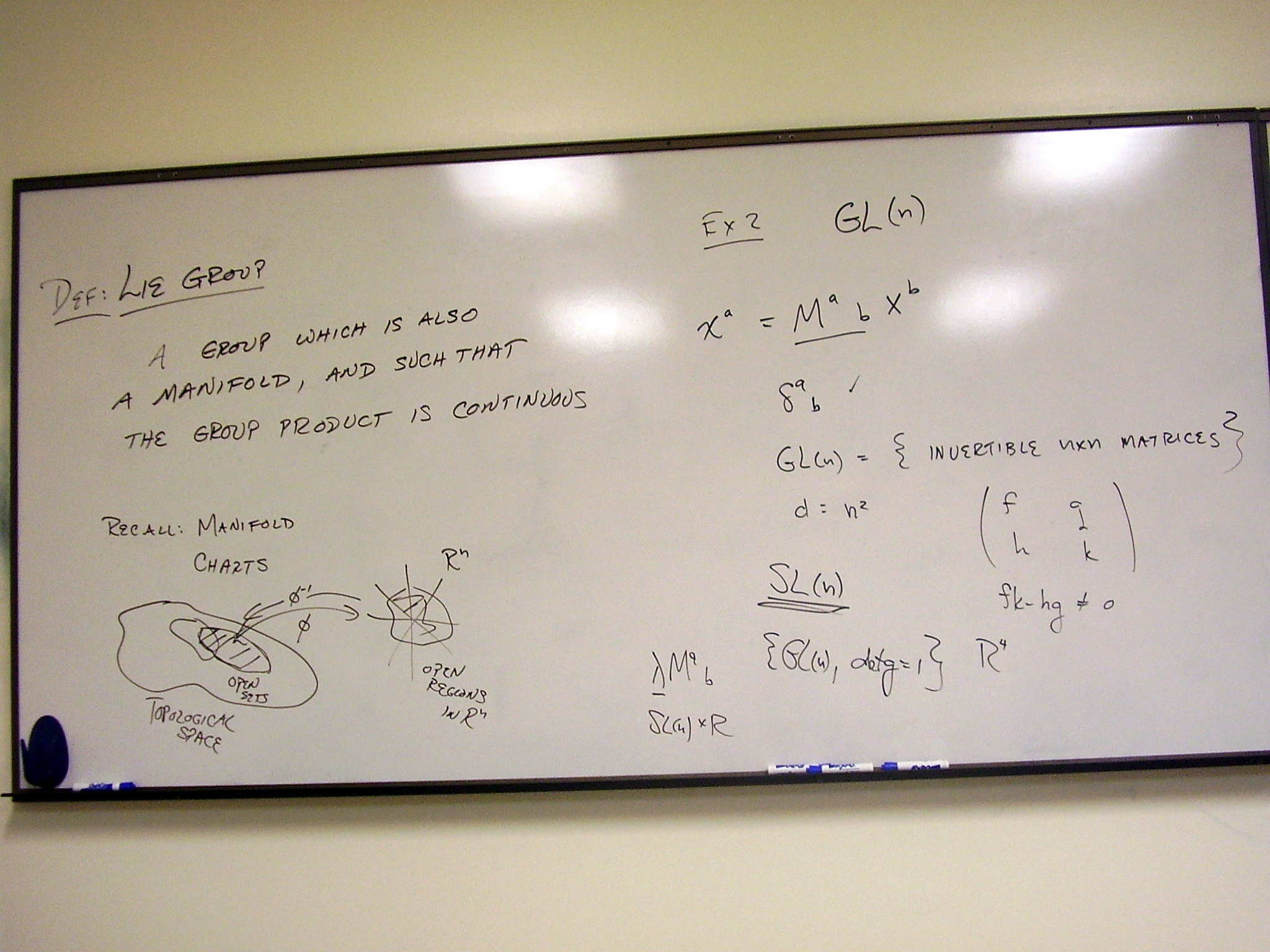
Symplectic, Sp(2n), and
complex groups (GL(n,C), SL(n,C), U(n), SU(n)).
An important example:
SL(2,C), the Lorentz group
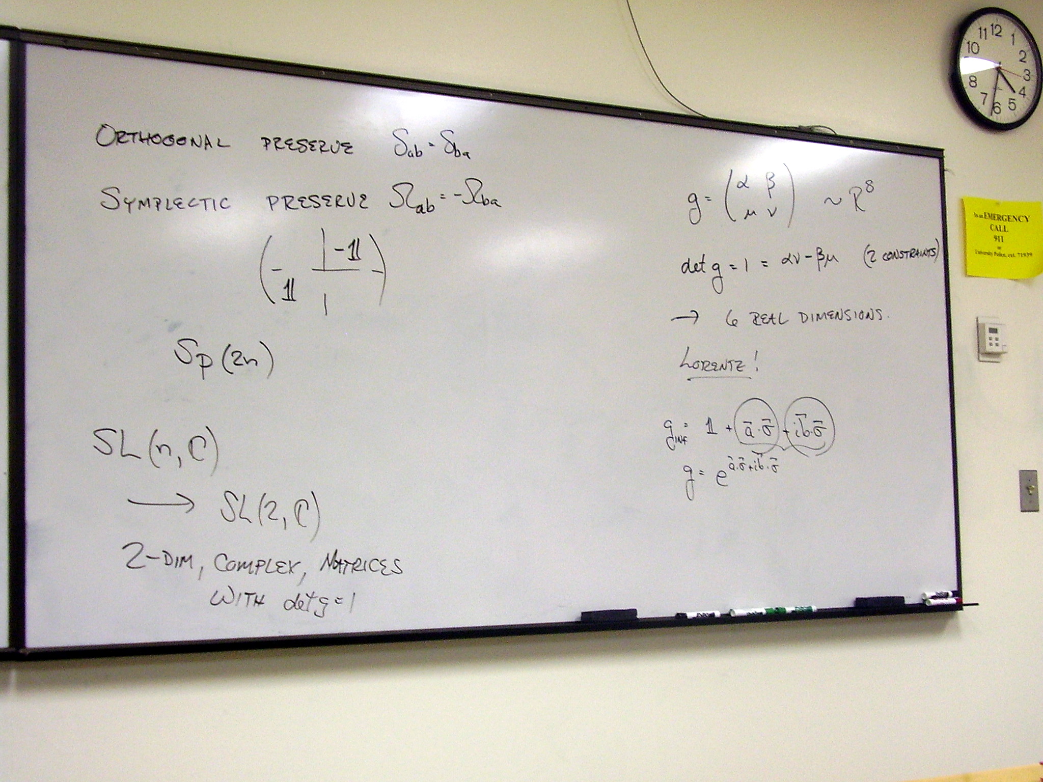
SL(2,C) and Lorentz
transformations
These complex vectors are
spinors:
Pseudo-orthogonal groups
preserve metrics with “timelike” directions:
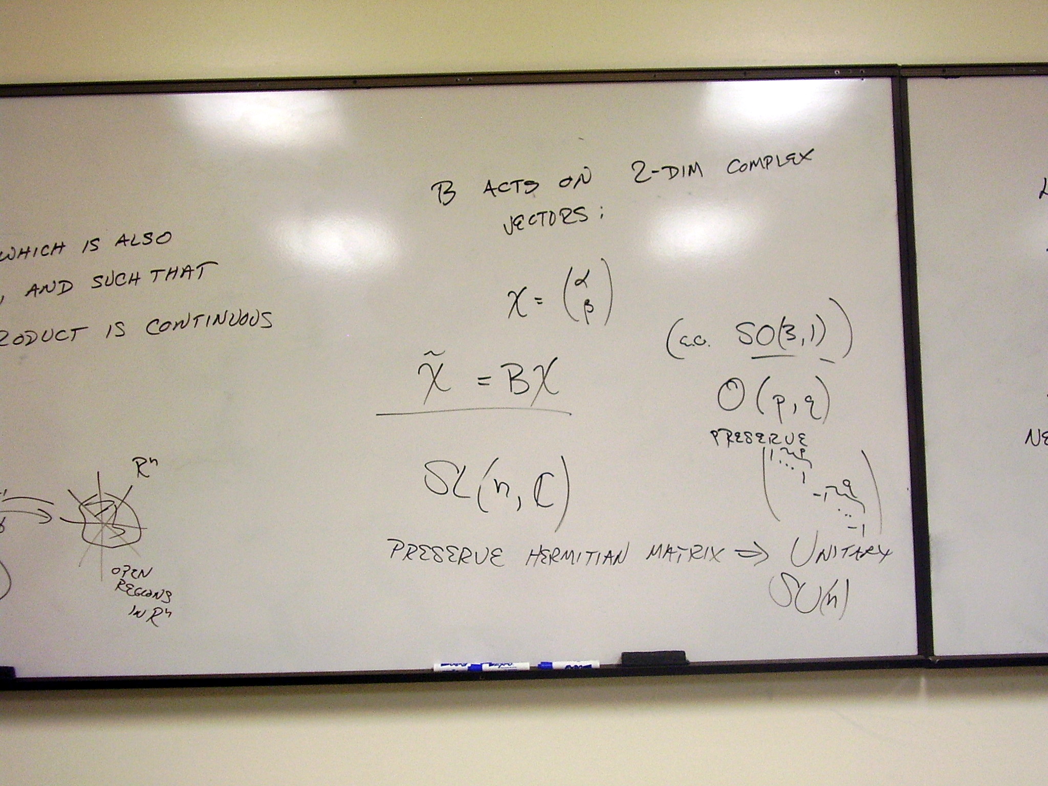
Friday, January 23,
2009
Lecture:
Examples of Lie groups
Two ways to show the
covariance of the divergence expression for the Maxwell field: easy, elegant
and quasi-satisfying,
or longer, messier, but
definitely complete:
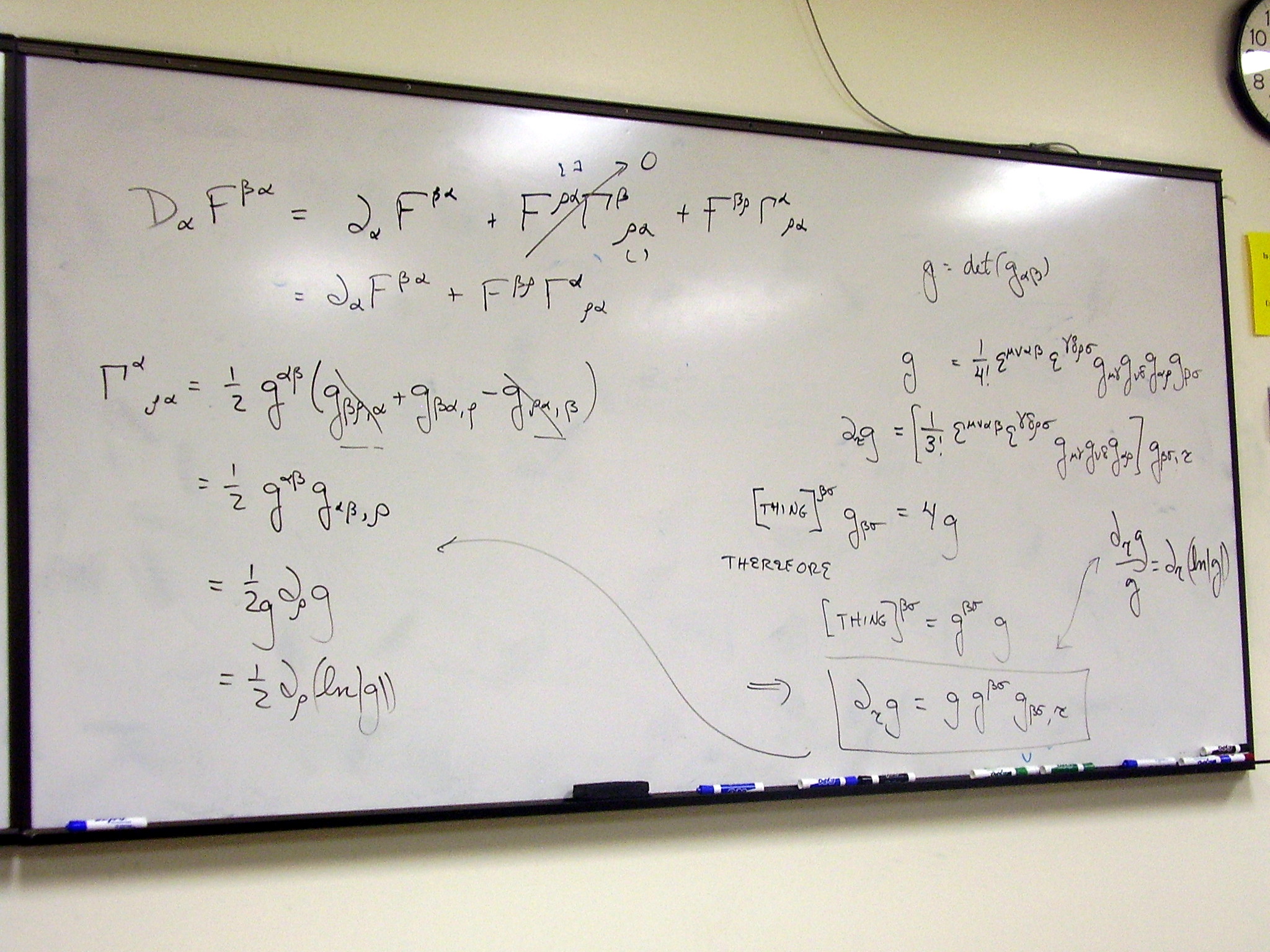
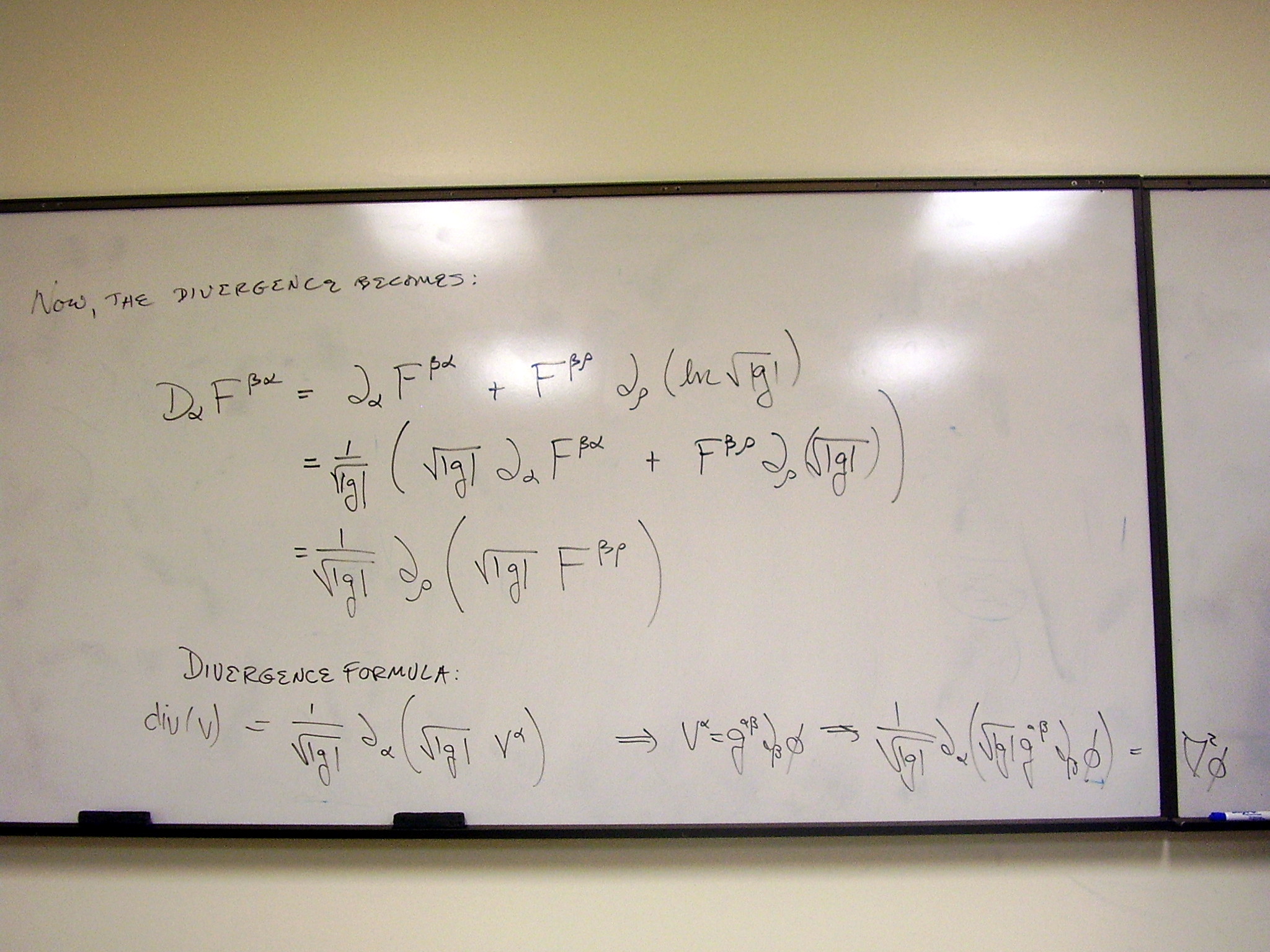
With a little care, we can
write the divergence formula using orthonormal frames:
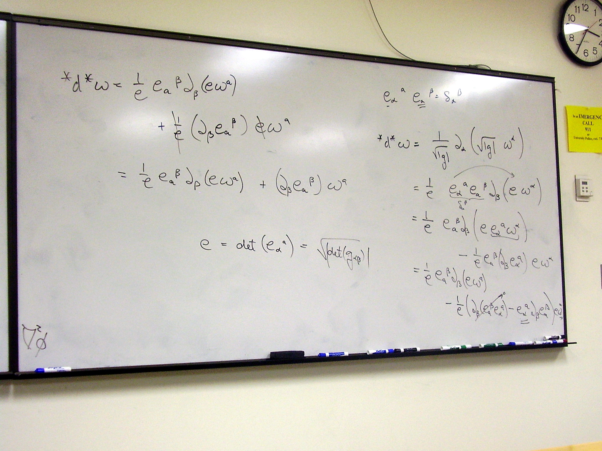
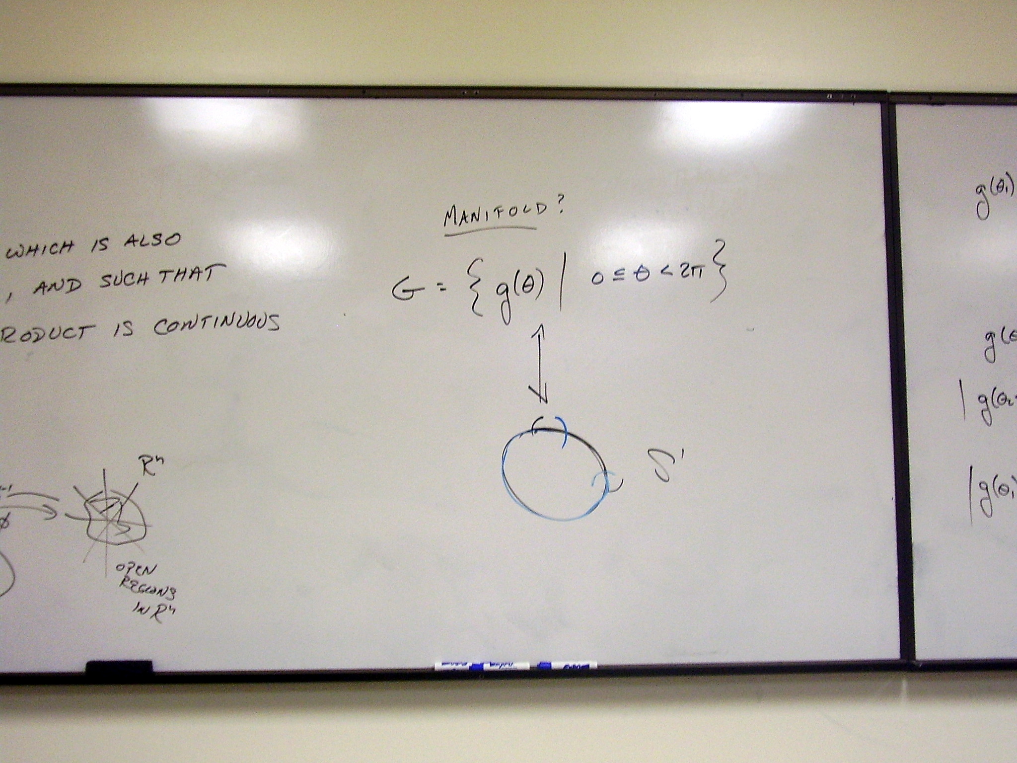
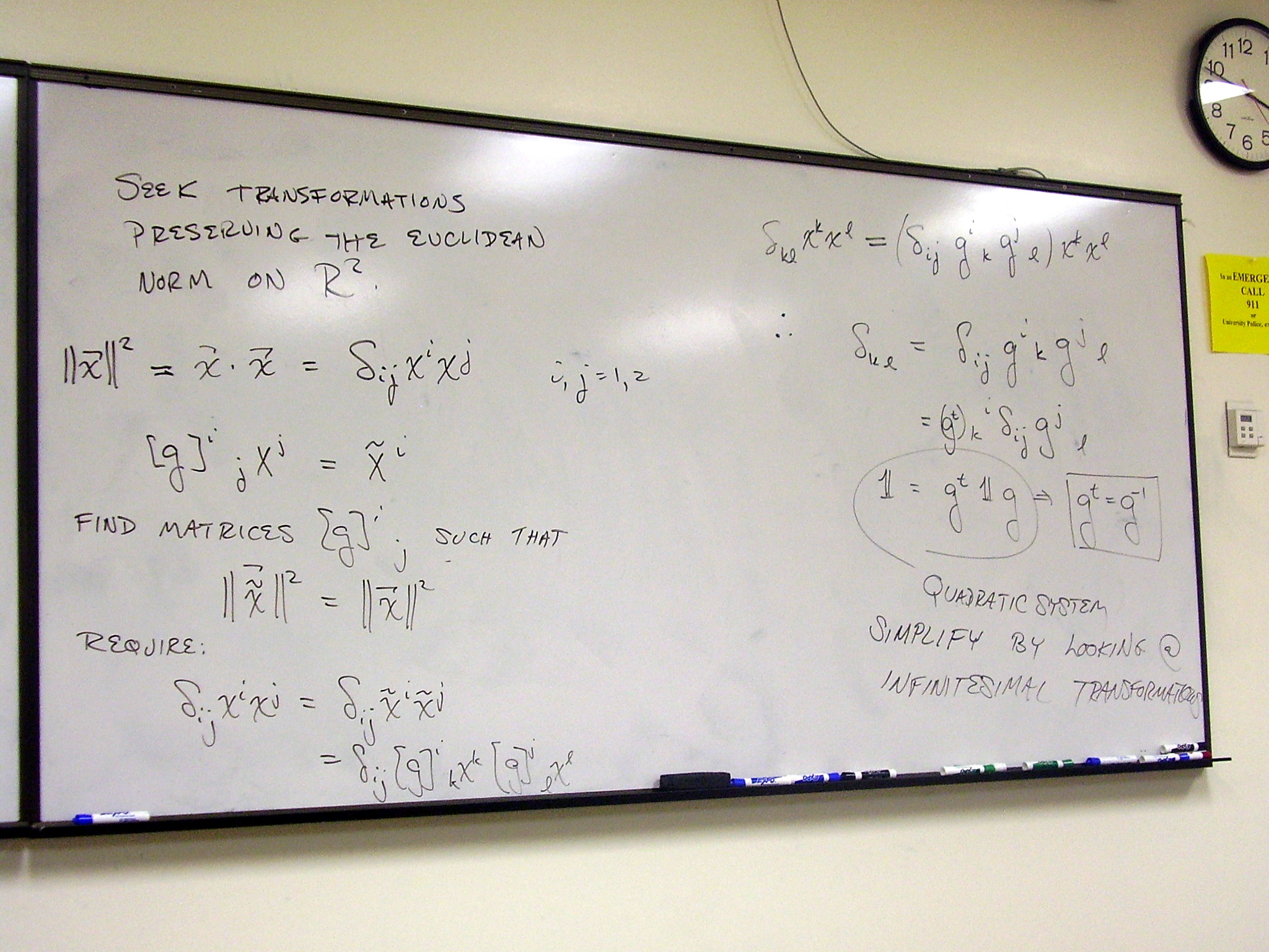
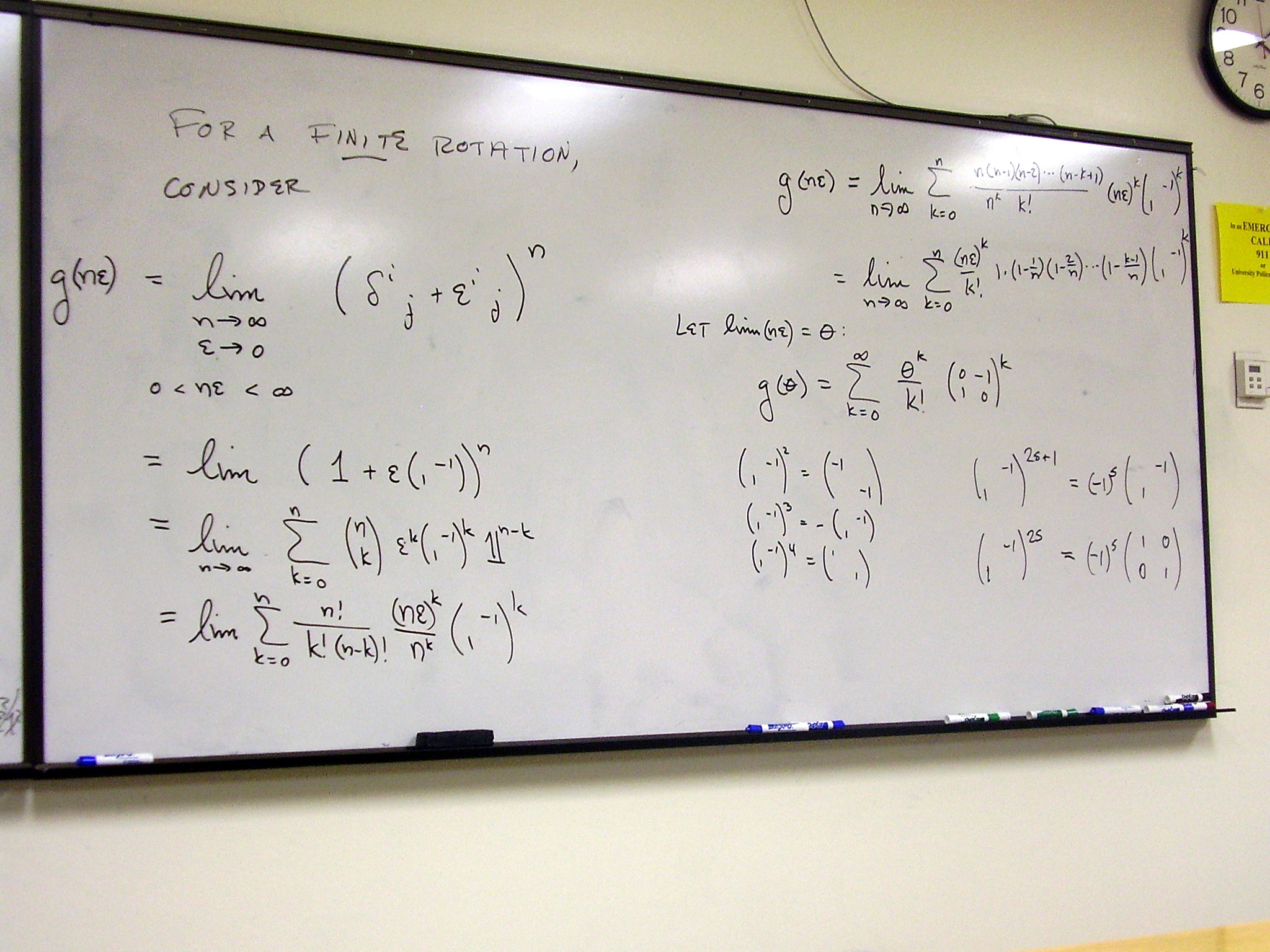
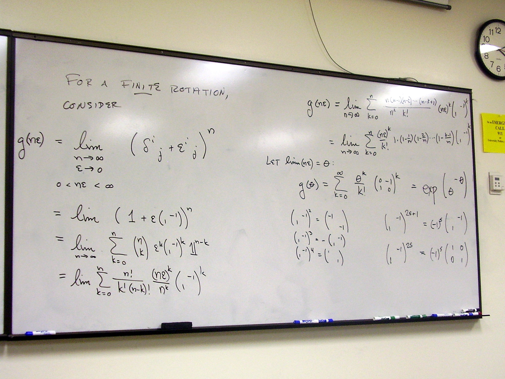
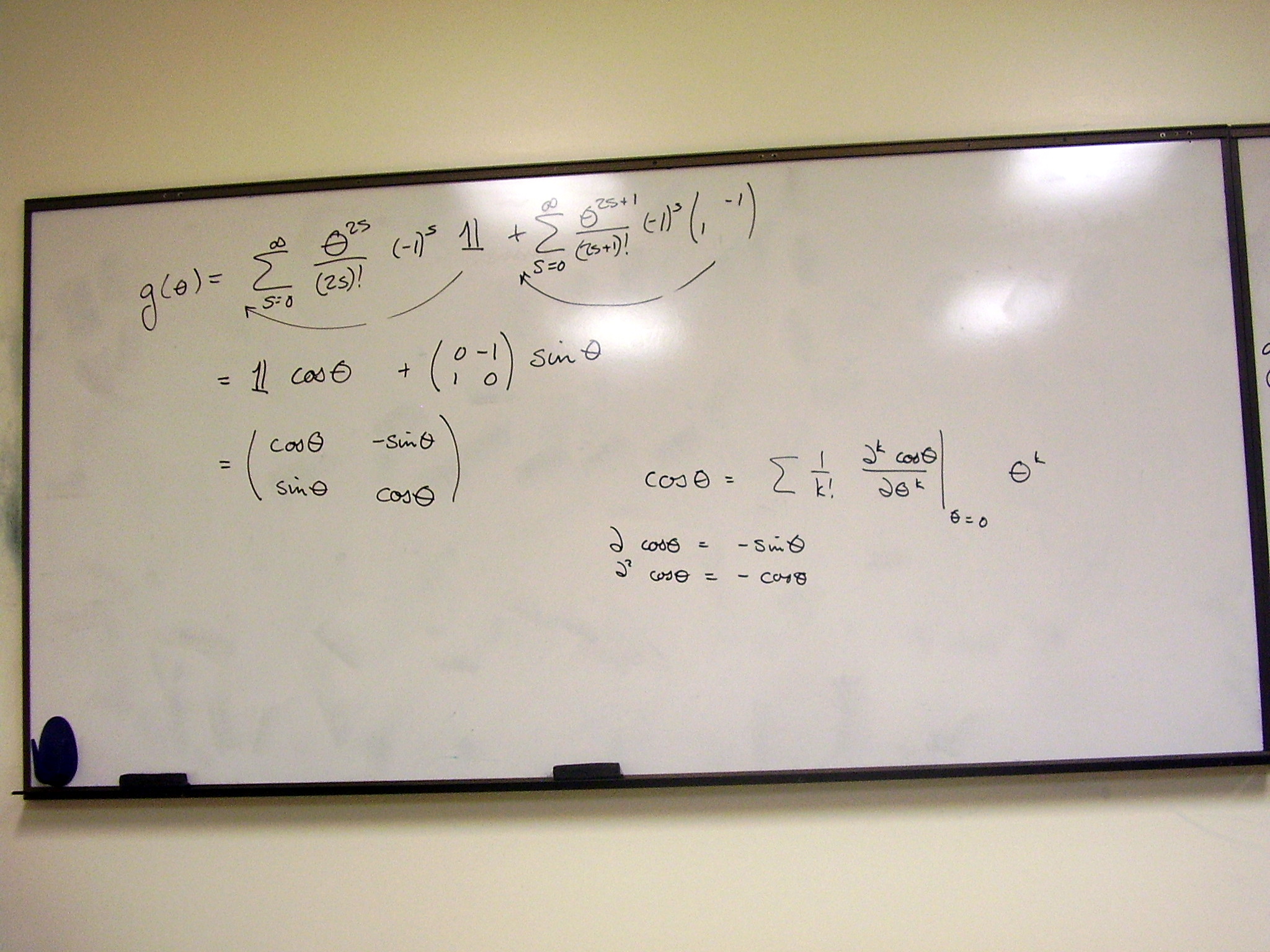
Example of a Lie group:
SO(2). Define the group by what it
leaves invariant and use this condition to find the general form of all (in
this case only one) infinitesimal transformations. By combining many
infinitesimal transformations – leading to the exponential of an
arbitrary real multiple of our infinitesimal form – we recover the form
of the general group element. The real multiple gives us the parameterization
of the group (or, equivalently, the chart from the group manifold into the
reals).
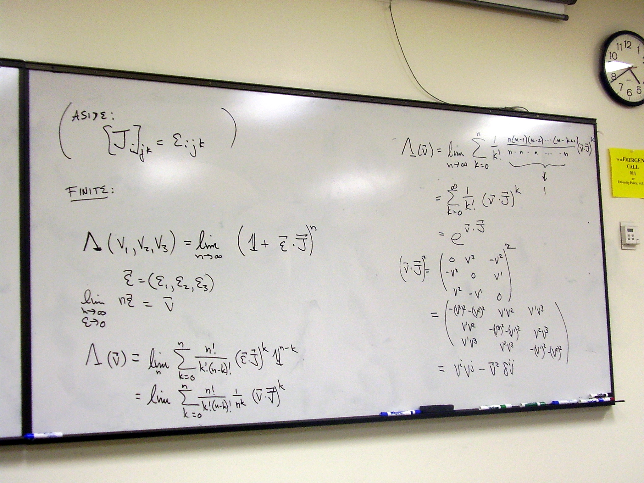
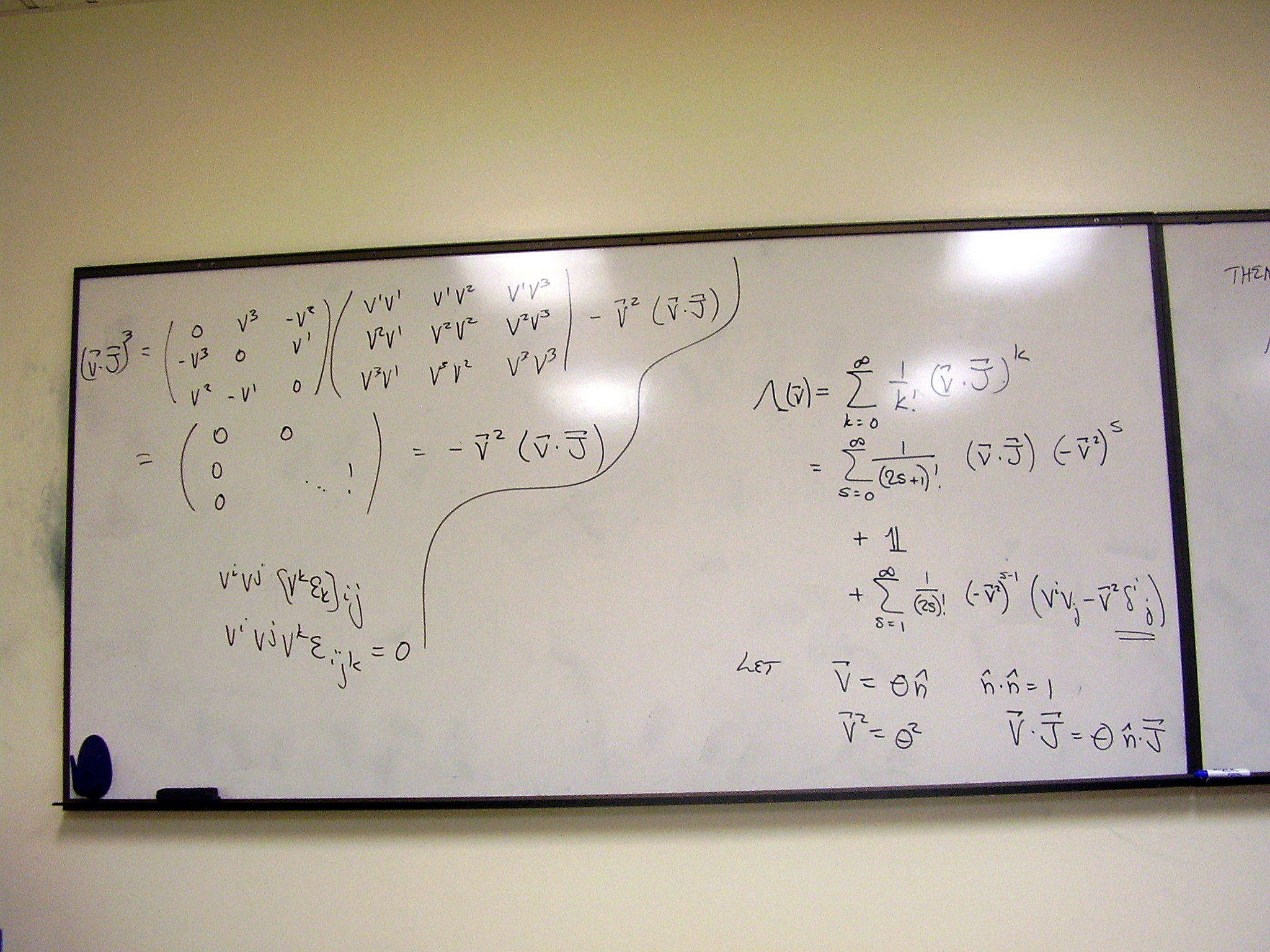
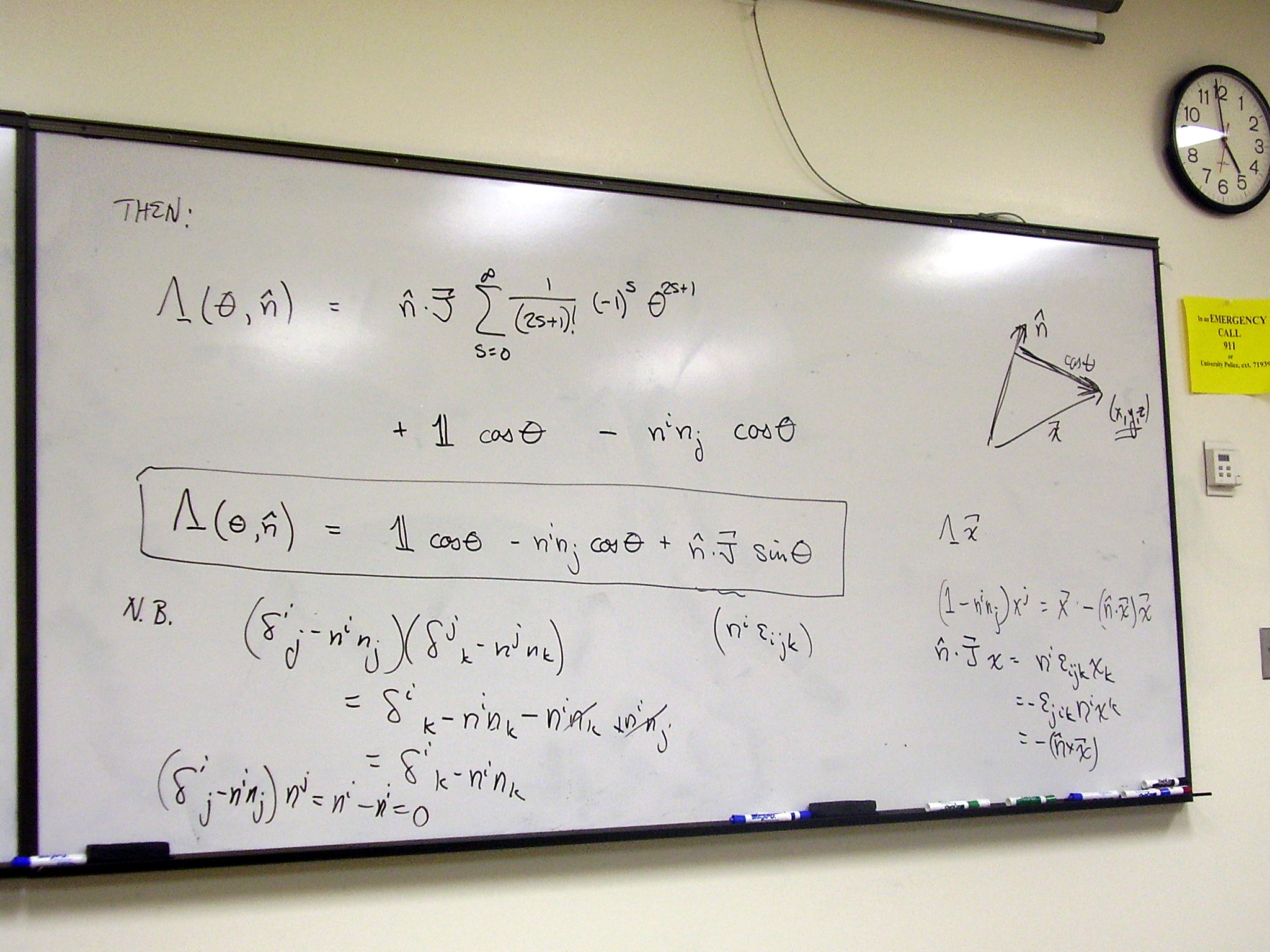
Example of a Lie group:
SO(3). The same procedure applied in 3 dimensions. This time there are three
independent transformations, and there are three infinitesimal “generators” of
the group – any three independent antisymmetric matrices. Group elements
are given by exponentiating an arbitrary real linear combination of these three
matrices. If we write the three real parameters as an angle times a unit
3-vector, it is easy to see that the result describes a rotation by that angle
in the plane perpendicular to the unit vector.
Monday, January 26,
2009
(Audio of the lecture is
coursing through the upper atmosphere, turning slowly into thermal energy and
escaping into space.)
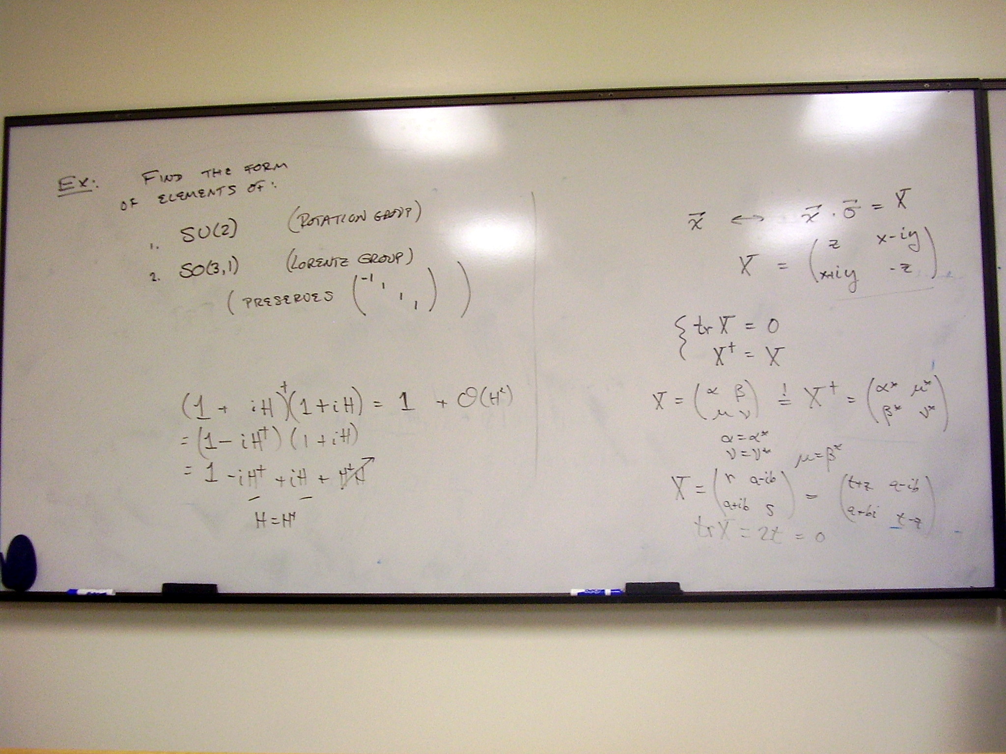
Exercise: Look at the Lie
groups SU(2) (rotations) and SO(3,1) (Lorentz).
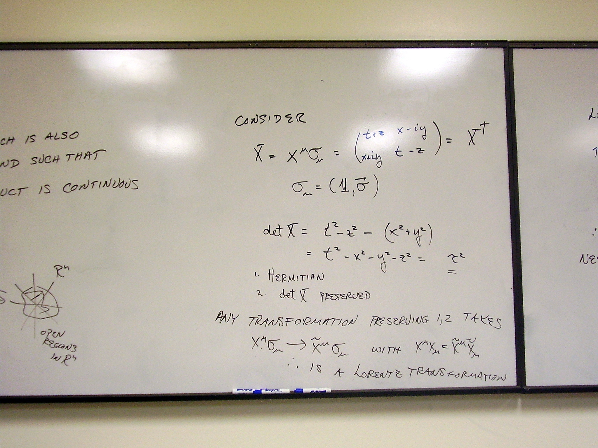
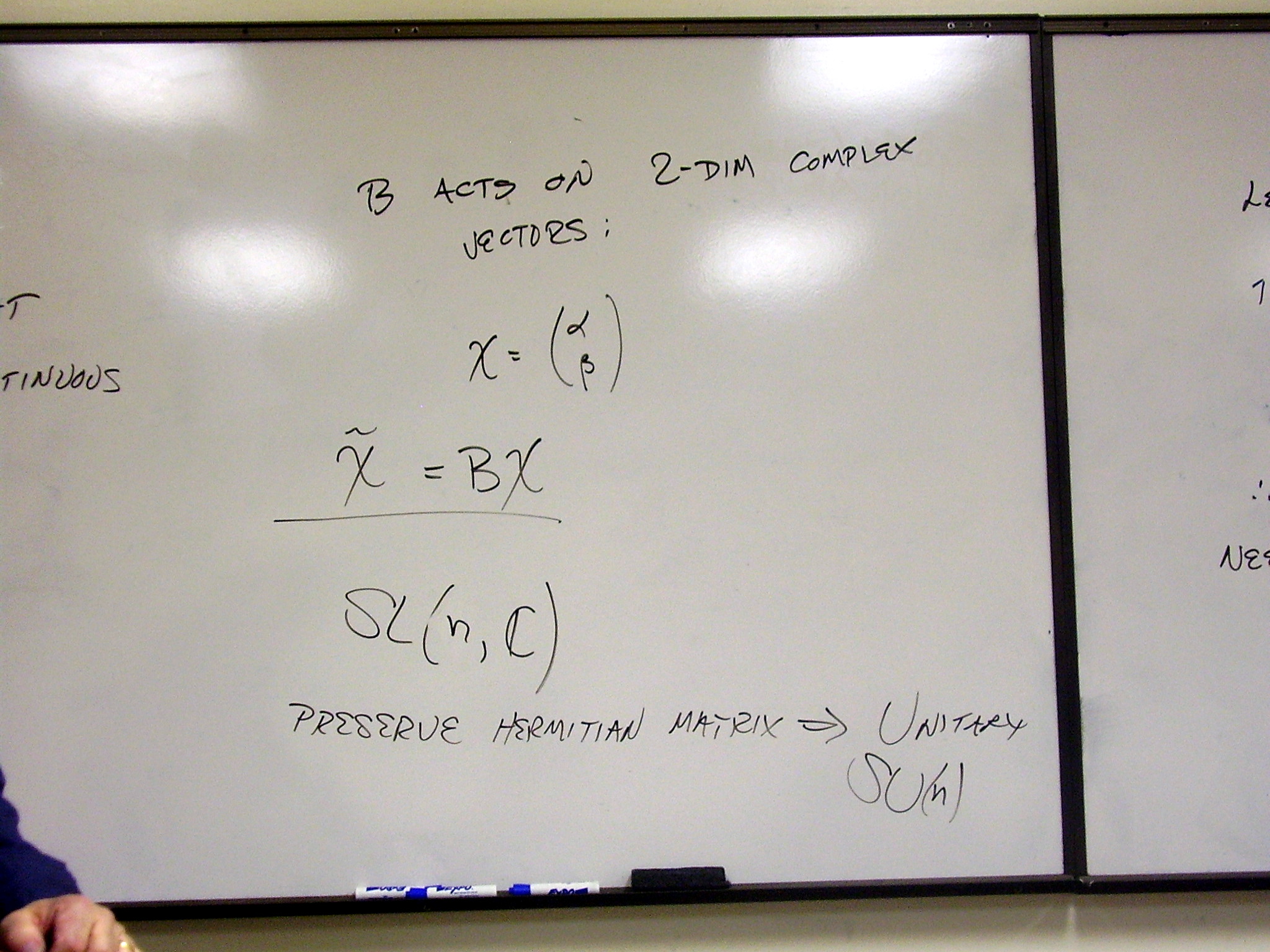
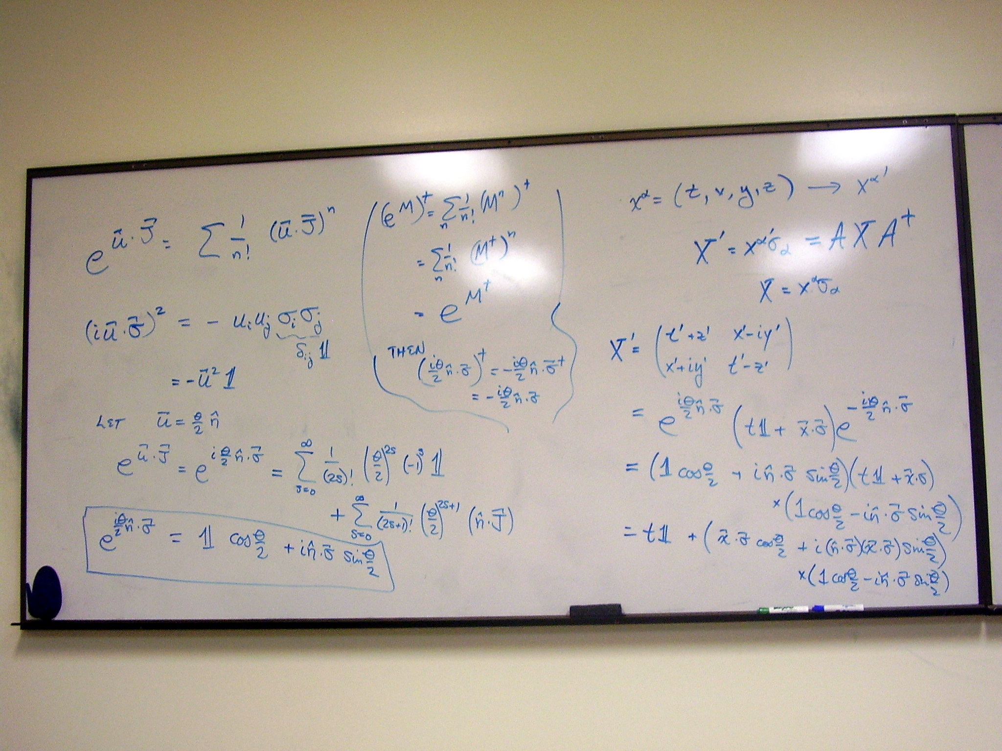
A proof that SU(2)
transformations produce 3 dimensional rotations. Writing a 3-vector, x, as a
traceless, Hermitian matrix X, a rotation will be any transformation that
preserves tracelessness, Hermiticity and the determinant of X:
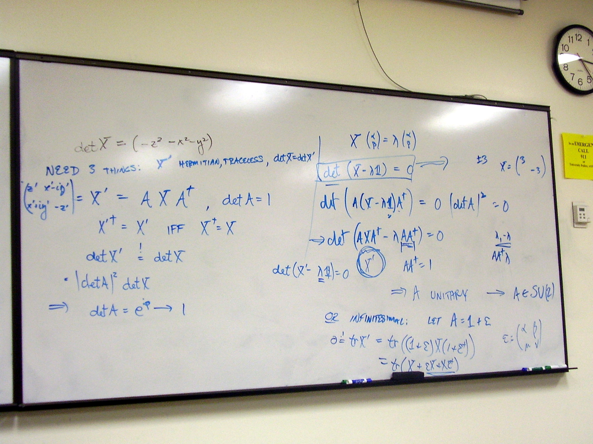
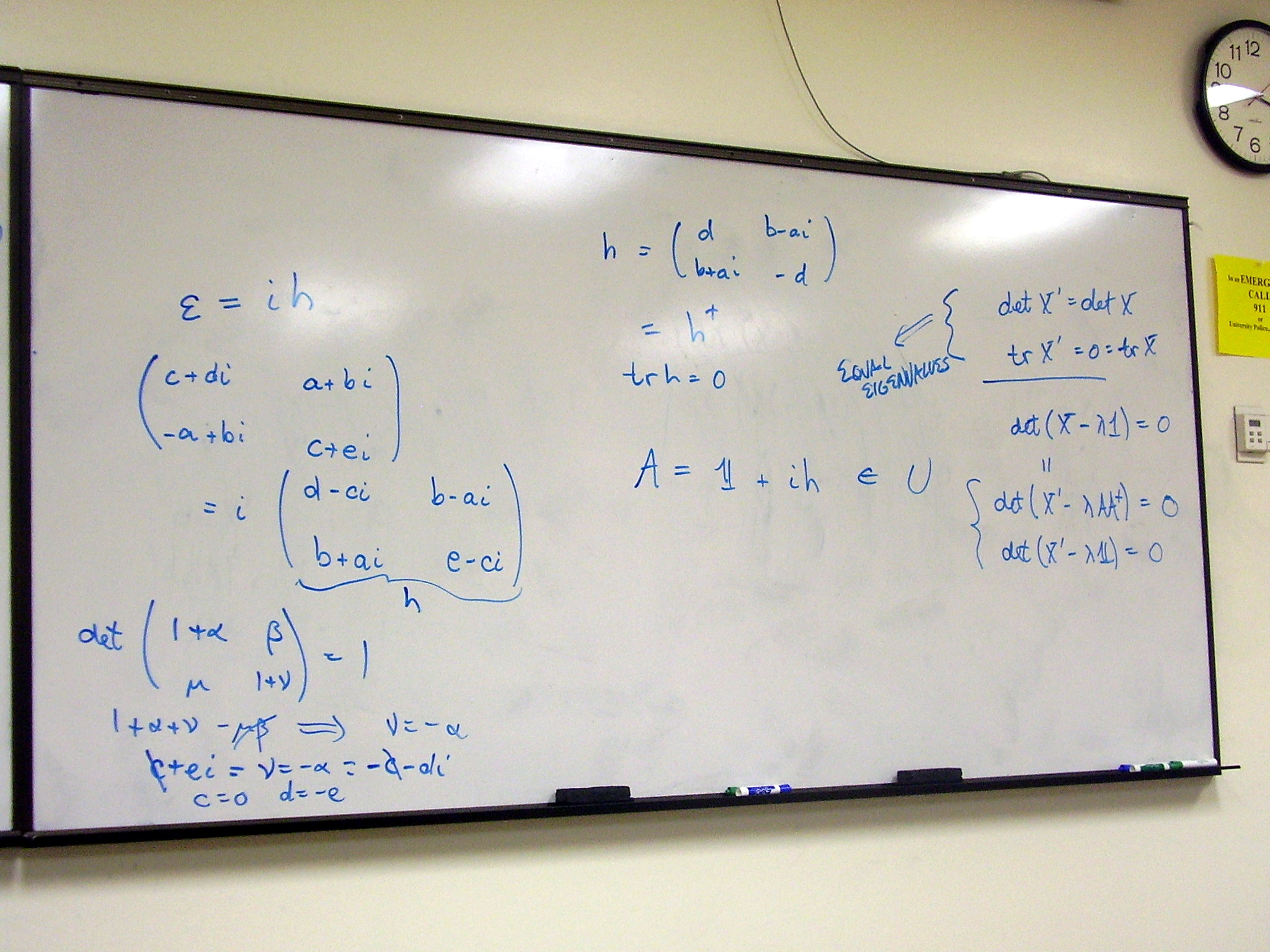
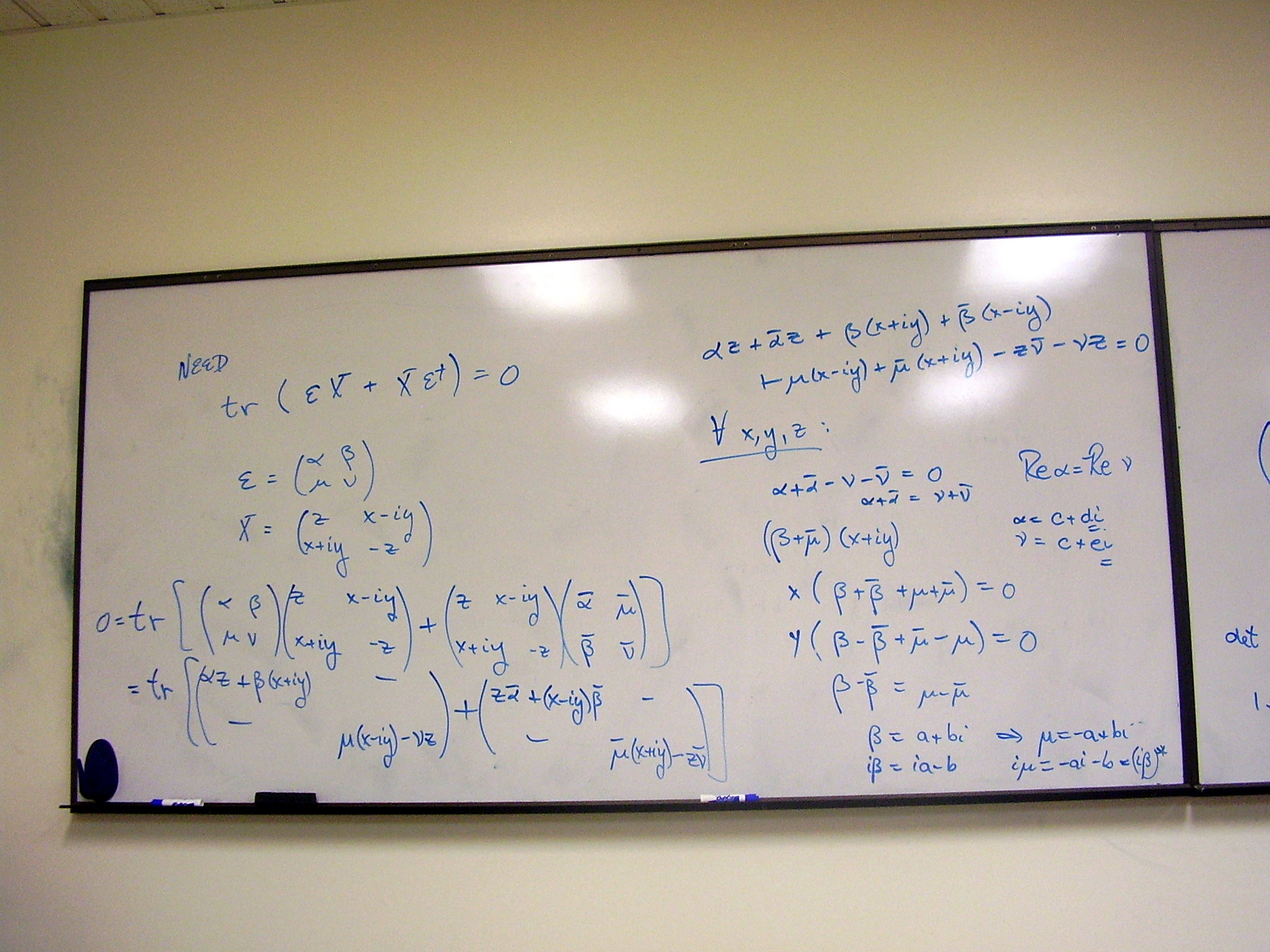
Revisiting SO(3): The
infinitesimal generators satisfy a closed, commutator algebra, and satisfy the
Jacobi identity:
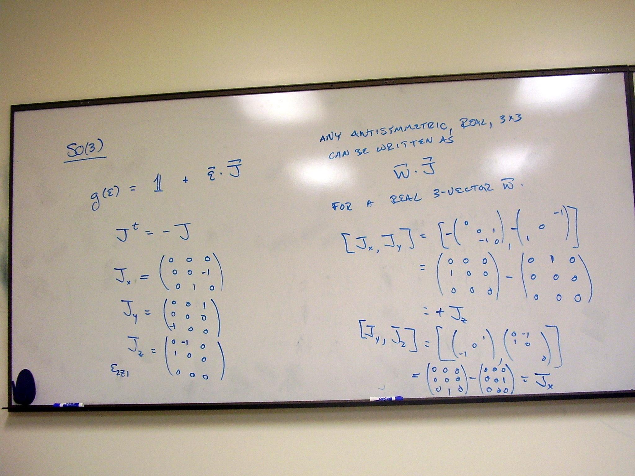
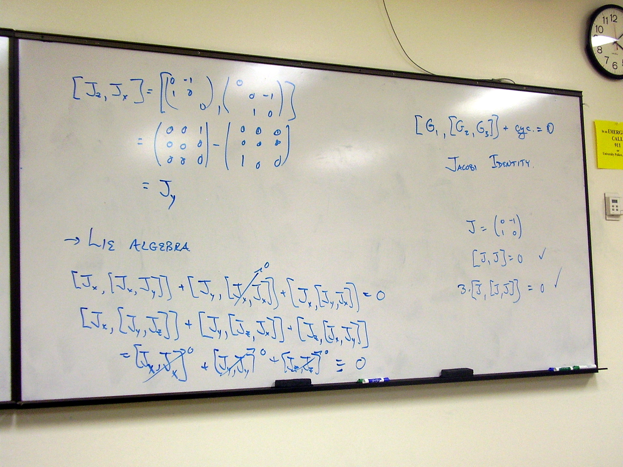
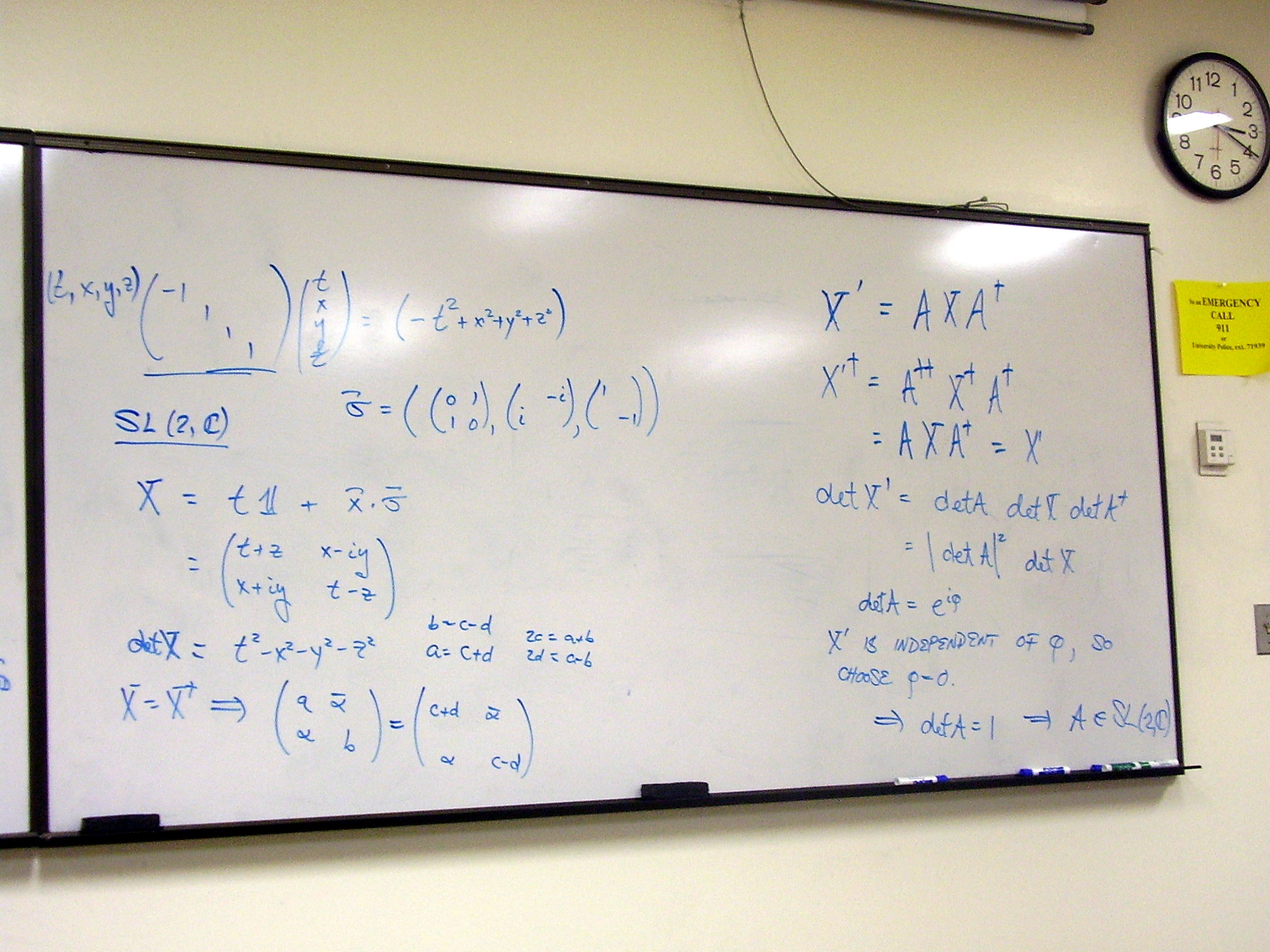
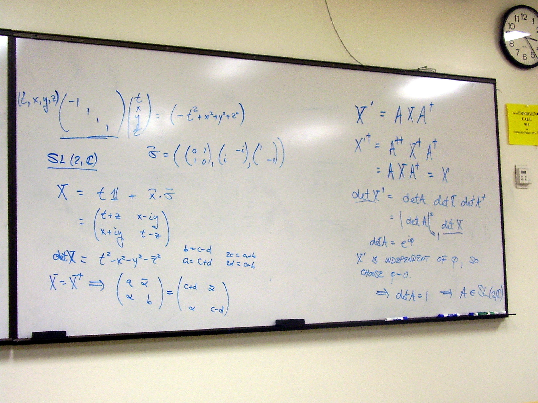
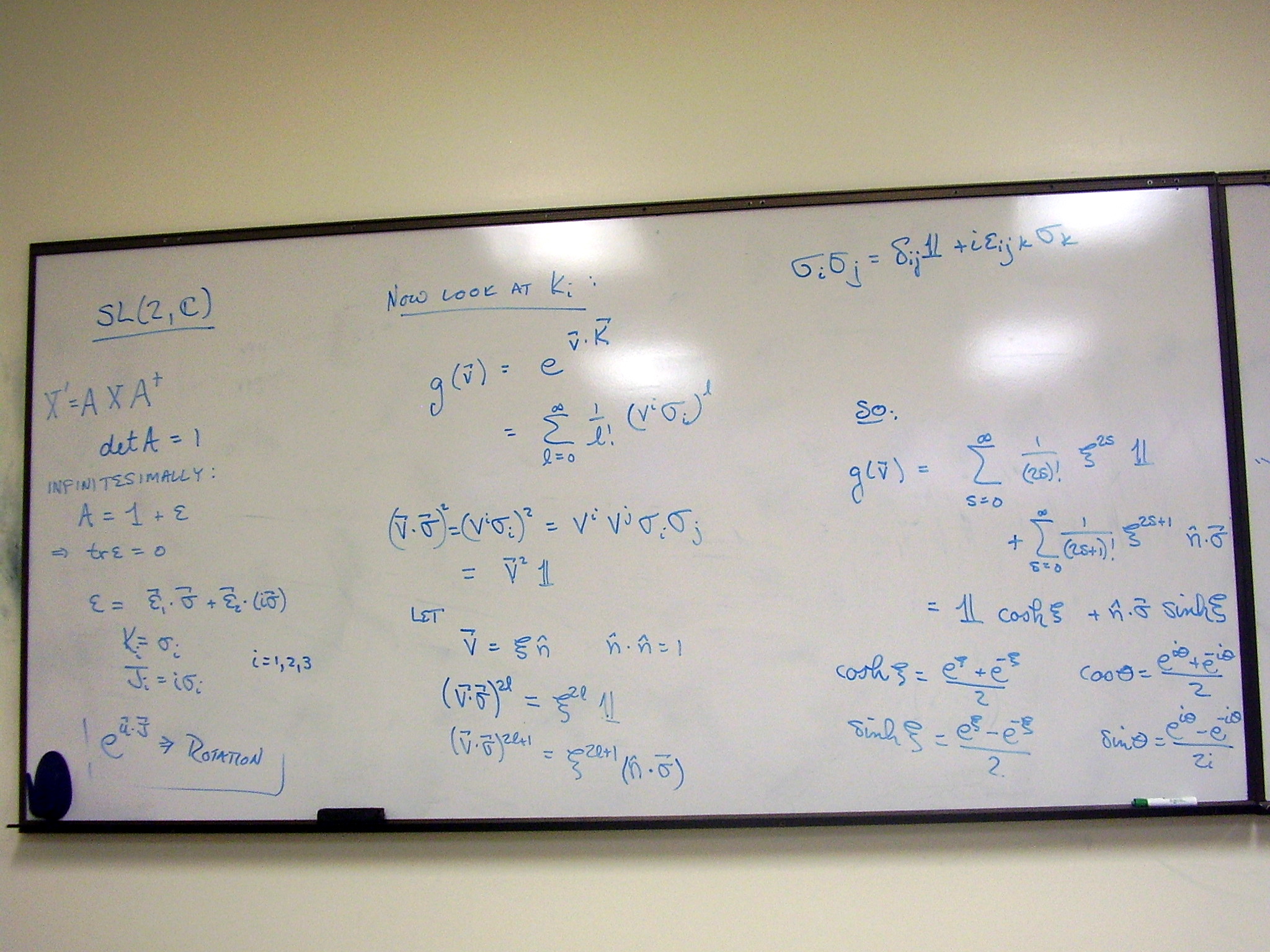
The Lie group SL(2,C).
Finding the infinitesimal generators and the commutation relations. A shortcut
to show that a finite transformation is given by the exponential.
Wednesday, January 28,
2009
A review of group
nomenclature and the classification of Lie groups
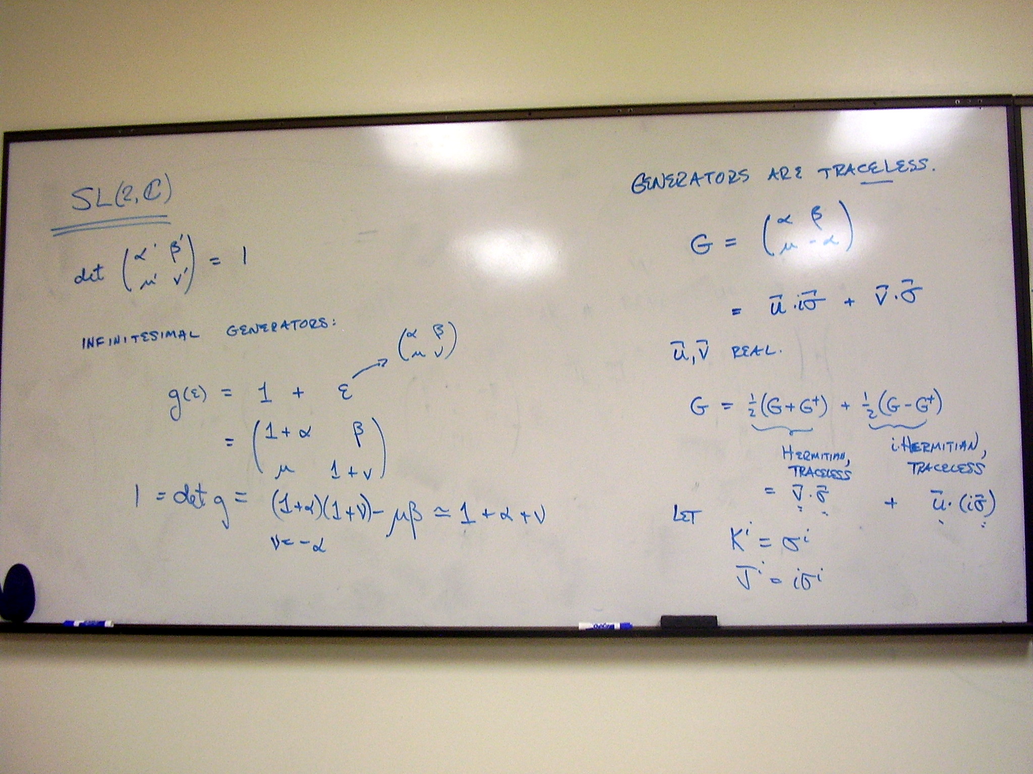
SL(2,C) (a spinor
representation of the Lorentz group). SL(2,C) preserves the Minkowski line
element.
Notice that the squared
norm of det(A) = 1
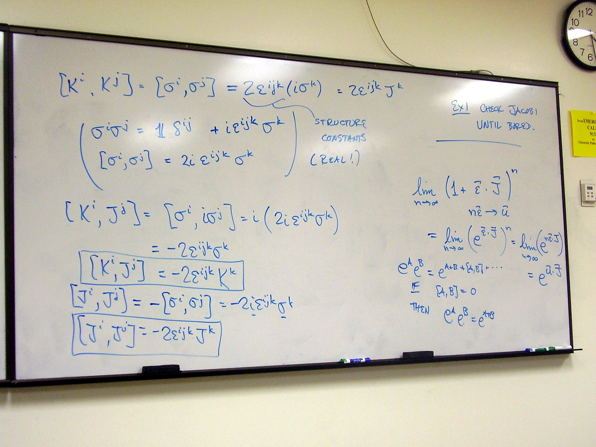
Finding the infinitesimal
generators:
Choosing a convenient
parameterization for the elements of the Lie algebra:
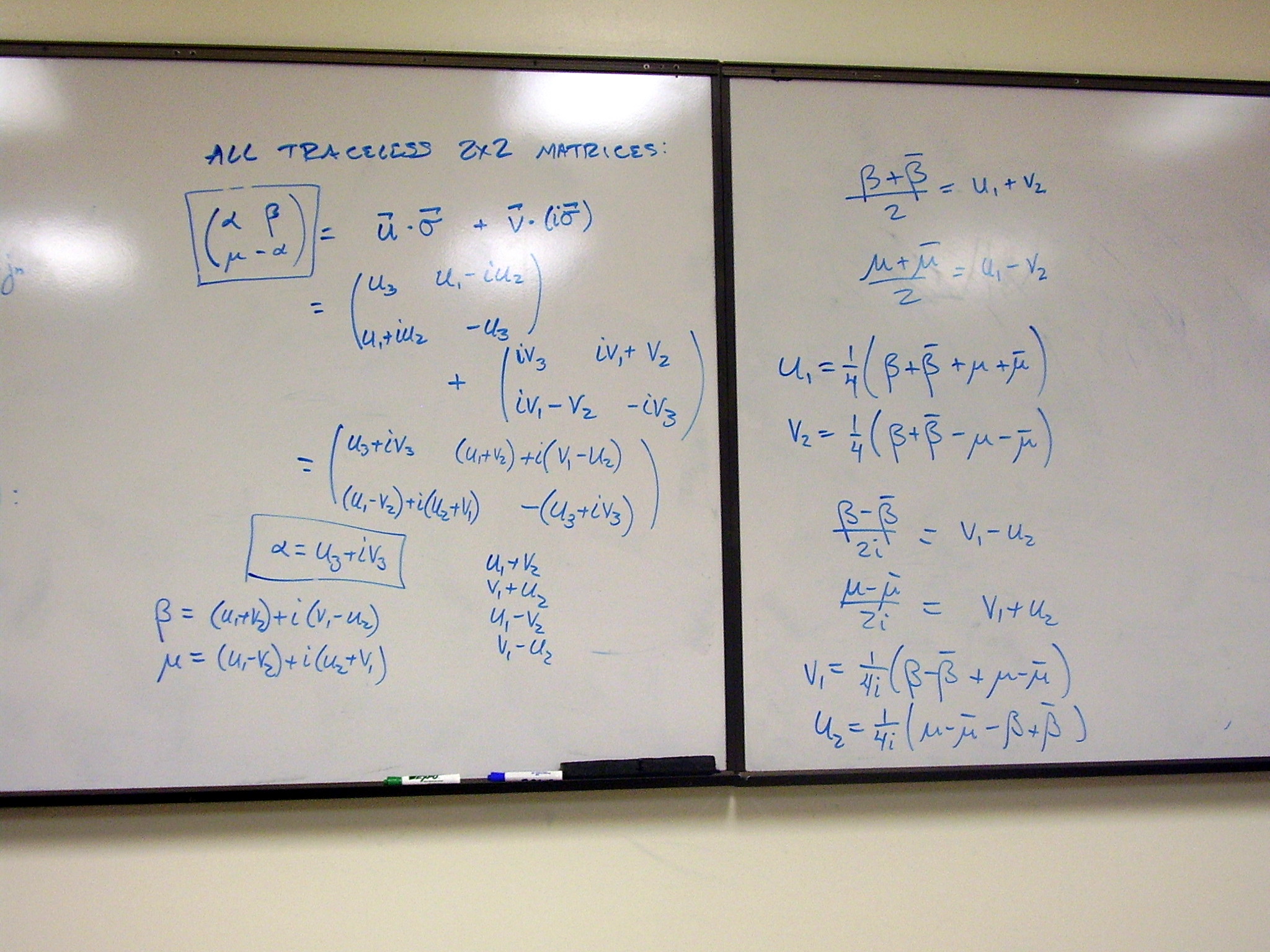
Defining the generators.
Recall that we checked the commutators and the Jacobi identity:
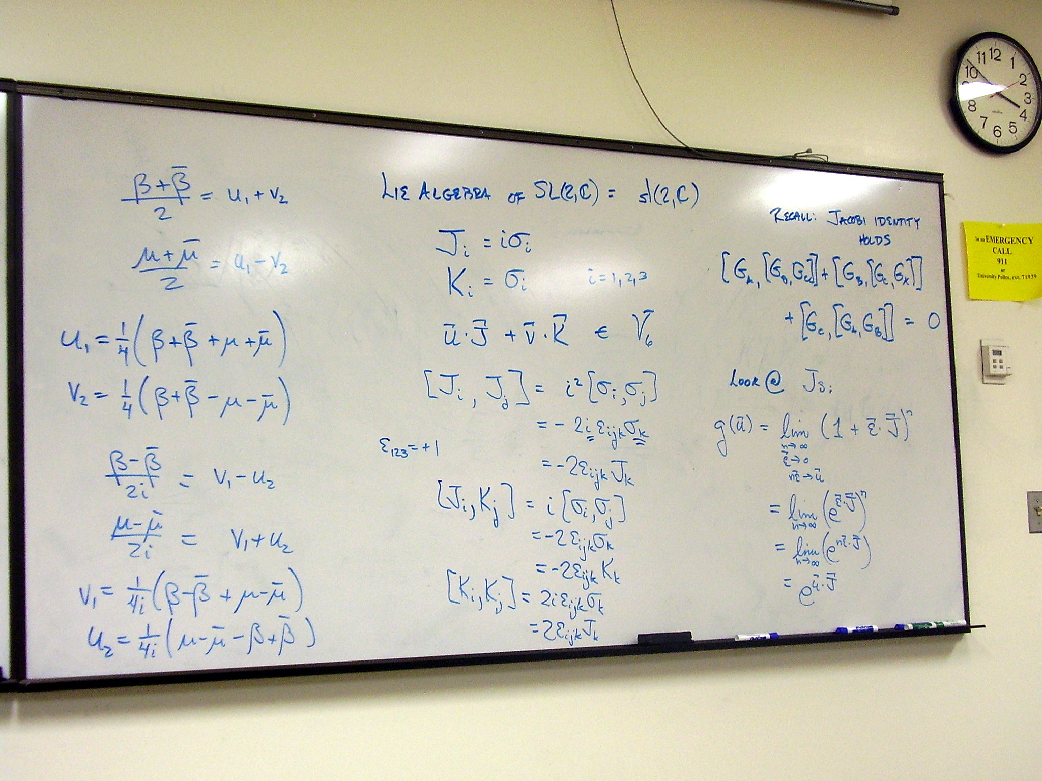
First look at the rotation
generators. Exponentiate.
Once we have a form fo the
exponential, we can rotate the spatial part of a 4-vector (written as a matrix,
X) to find a new 4-vector X’. To do this we use a similarity transformation.
Interpreting the result geometrically is not too difficult.
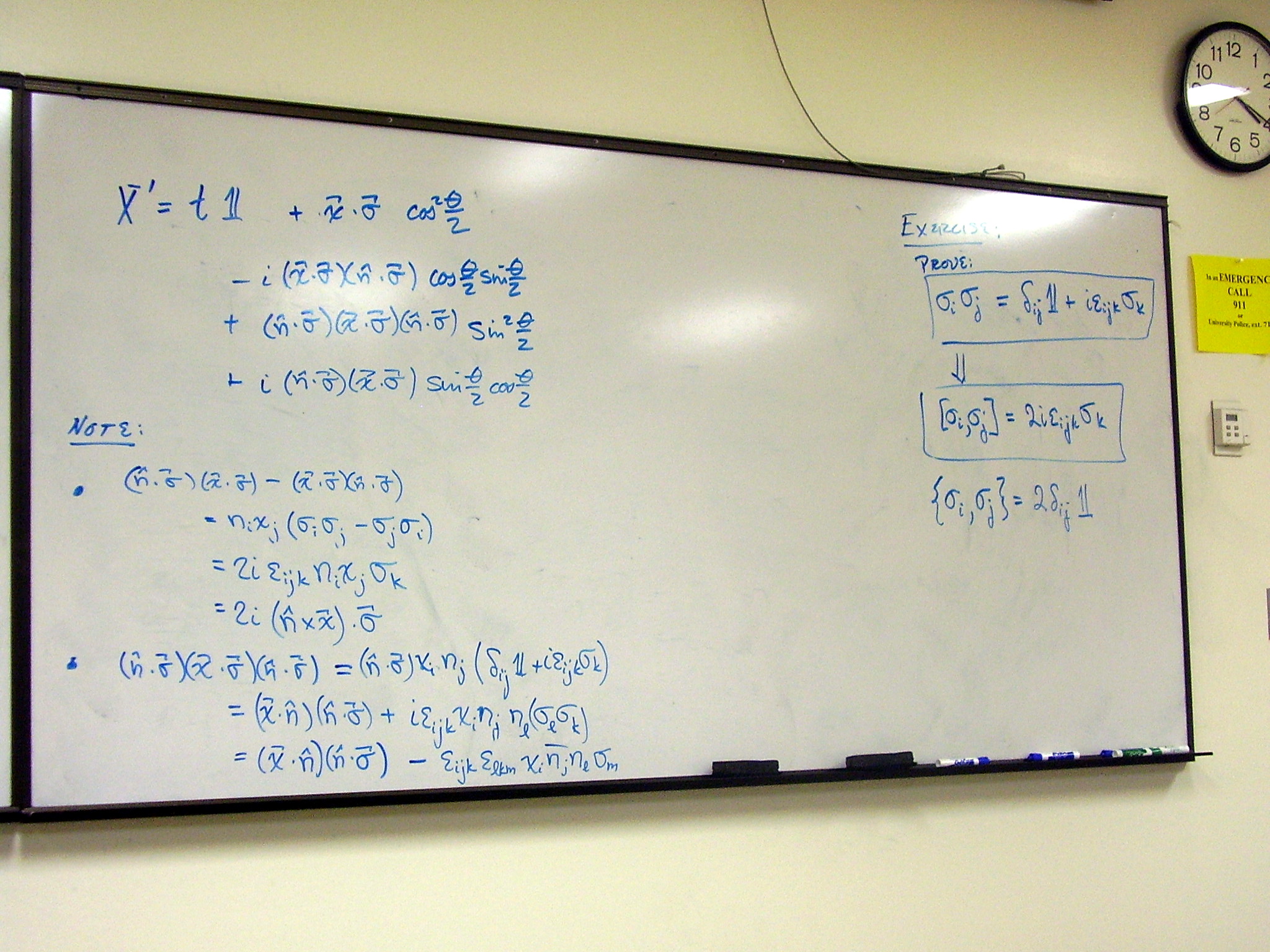
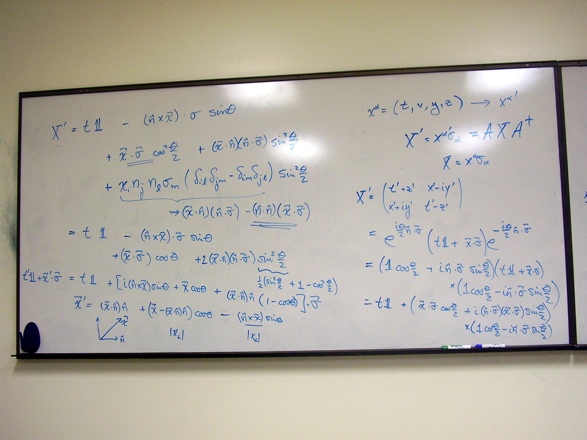
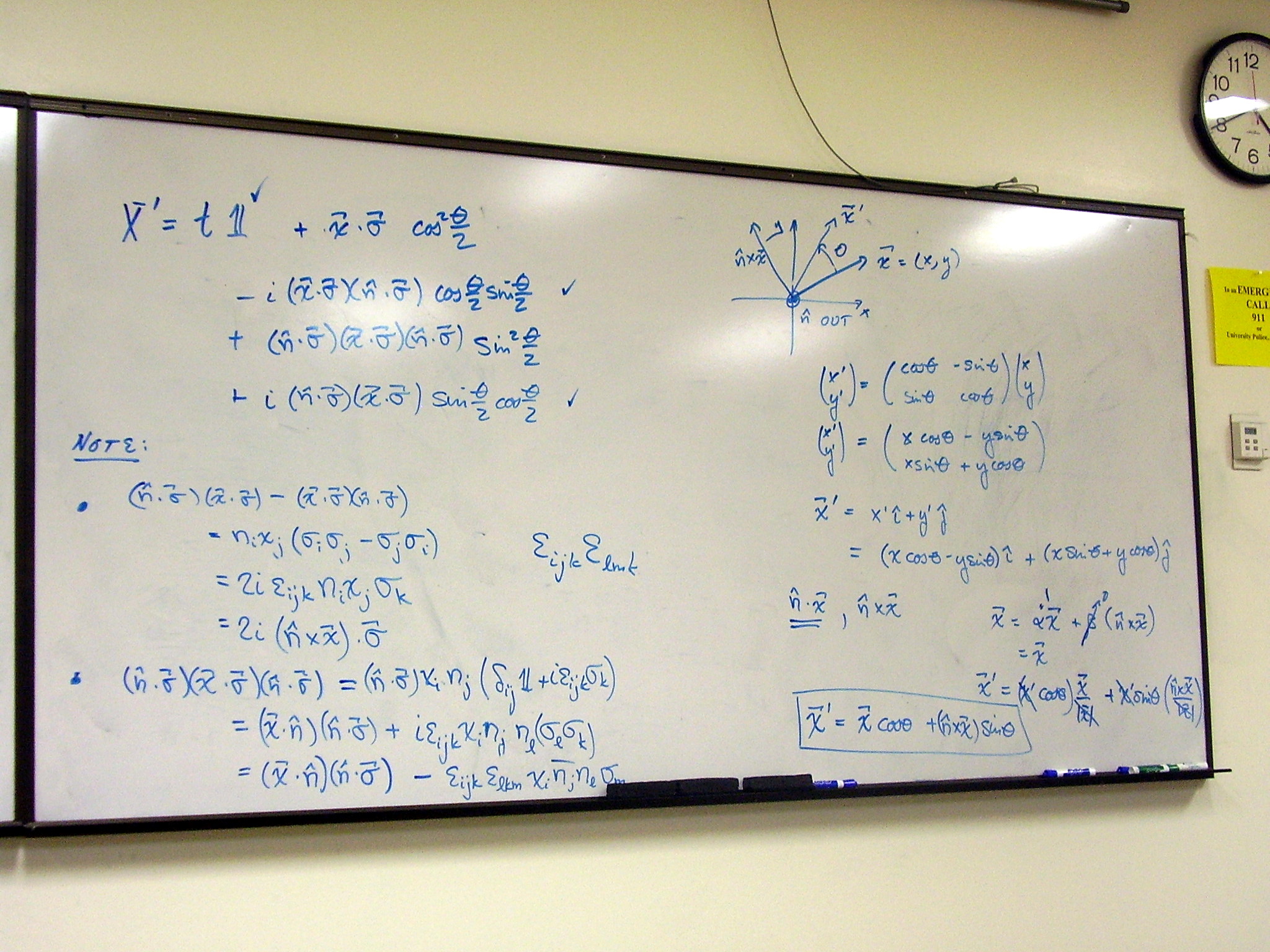
Friday, January 30,
2009
Lecture:
SL(2,C), continued. Boosts.
Continuing with the Lorentz
group, we exponentiate the infinitesimal generators of boosts. This time we get
hyperbolic functions instead of circular functions:
Comparing circular and
hyperbolic functions. Transforming a 4-vector:
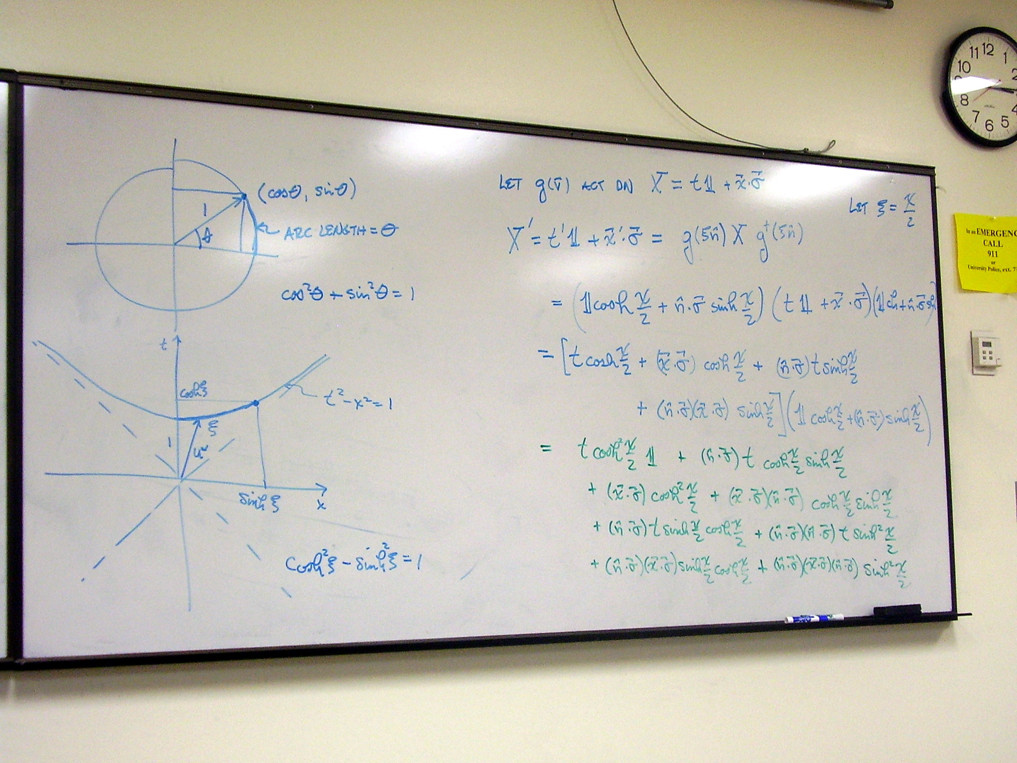
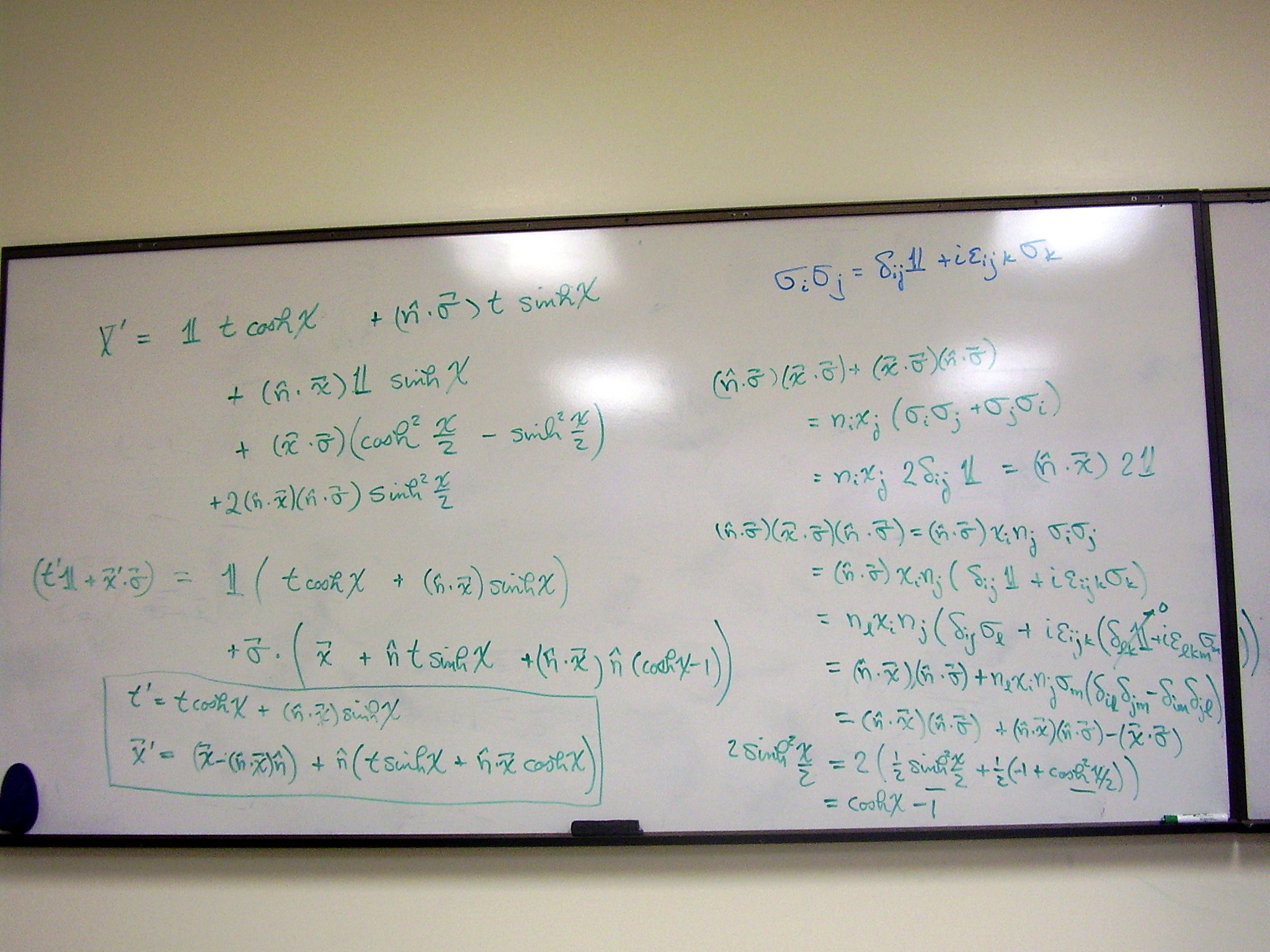
Specialize the answer to a
boost in the x-direction, and rewrite it in terms of the velocity:
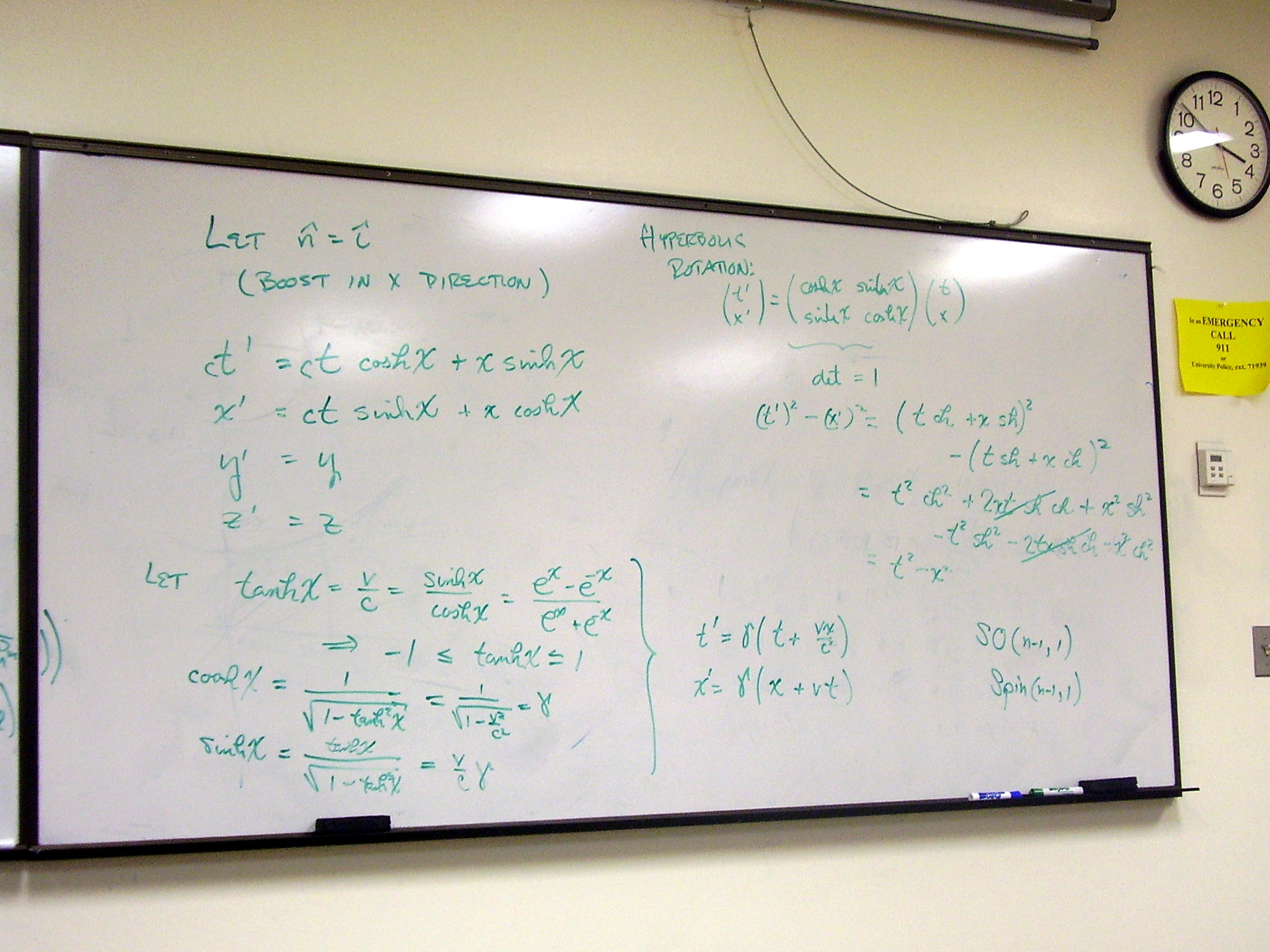
Monday, February 2,
2009
Lecture:
Lie groups: the formal development of the Lie algebra
Overview of the course; an
example using differential forms to derive the triple cross product;
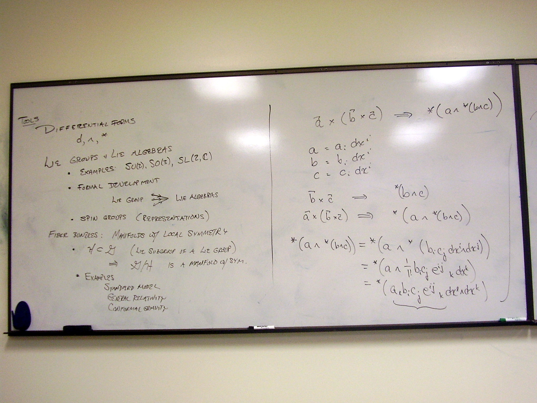
Triple cross product
continued; proving the usual formula for the dot product:
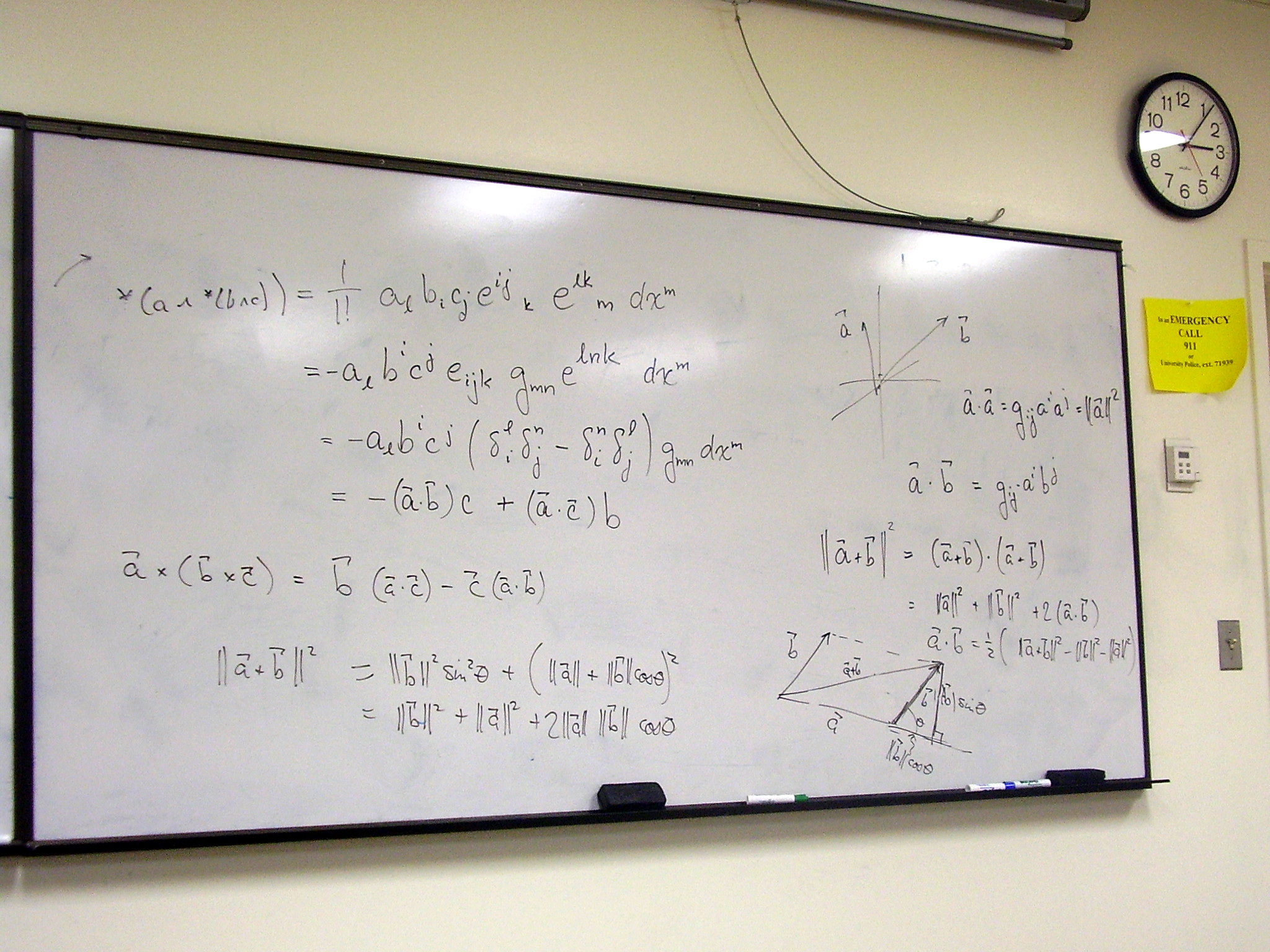
Statement of the theorem:
a Lie group gives rise to a Lie algebra. The Lie algebra is essentially the
tangent plane at the identity, and has a basis provided by the infinitesimal
generators of the group. An example: SO(3).
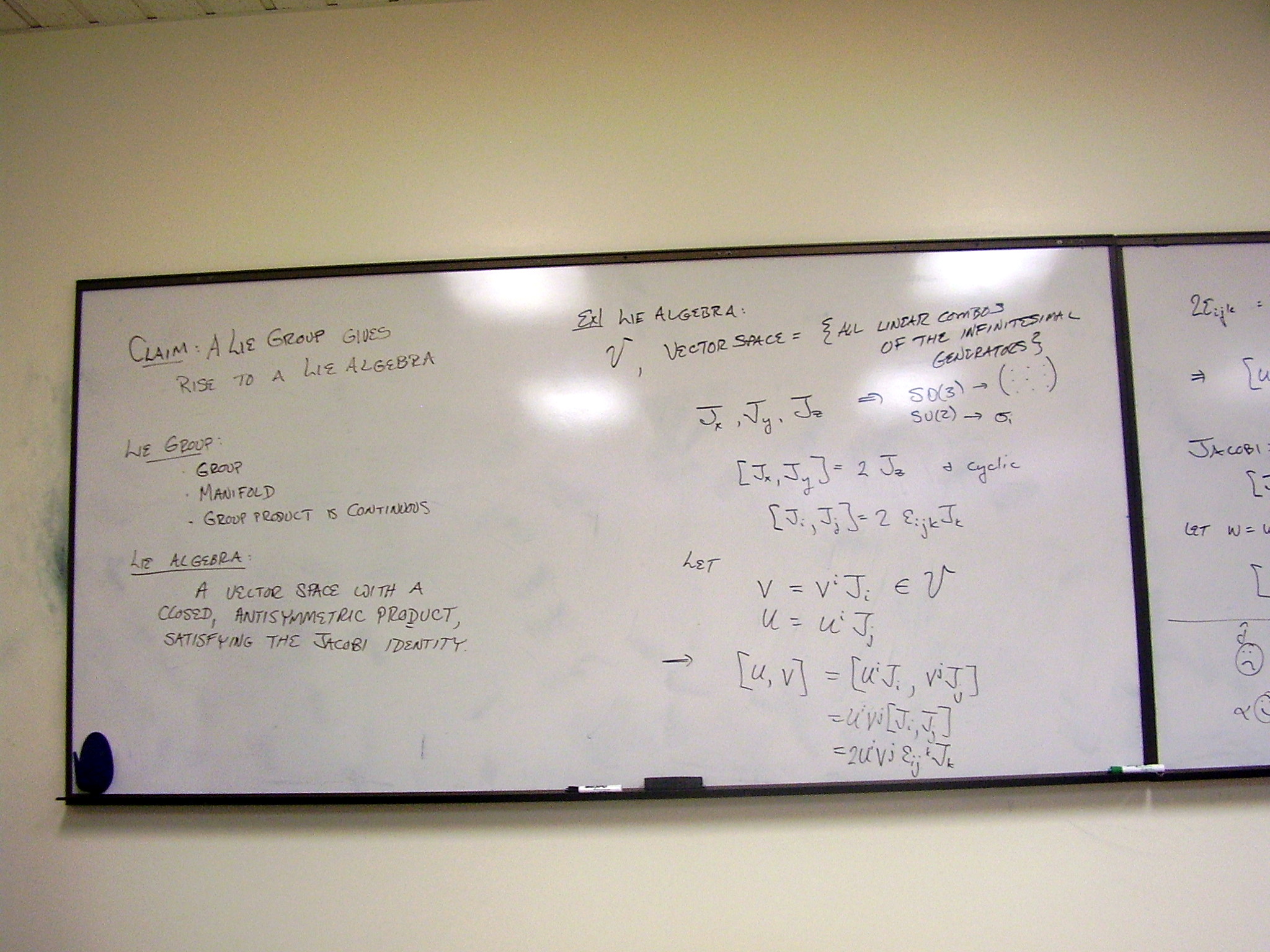
Expanding some group
elements and their inverses near the identity:
A particular product of
group elements and their inverses, expanded near the identity, will give us the
commutator. Closure of the group shows that the commutator closes. Notice that
the proof uses 3 of the group properties: closure, identity and inverse. The
result is so good, we’ve got it twice (g,h):
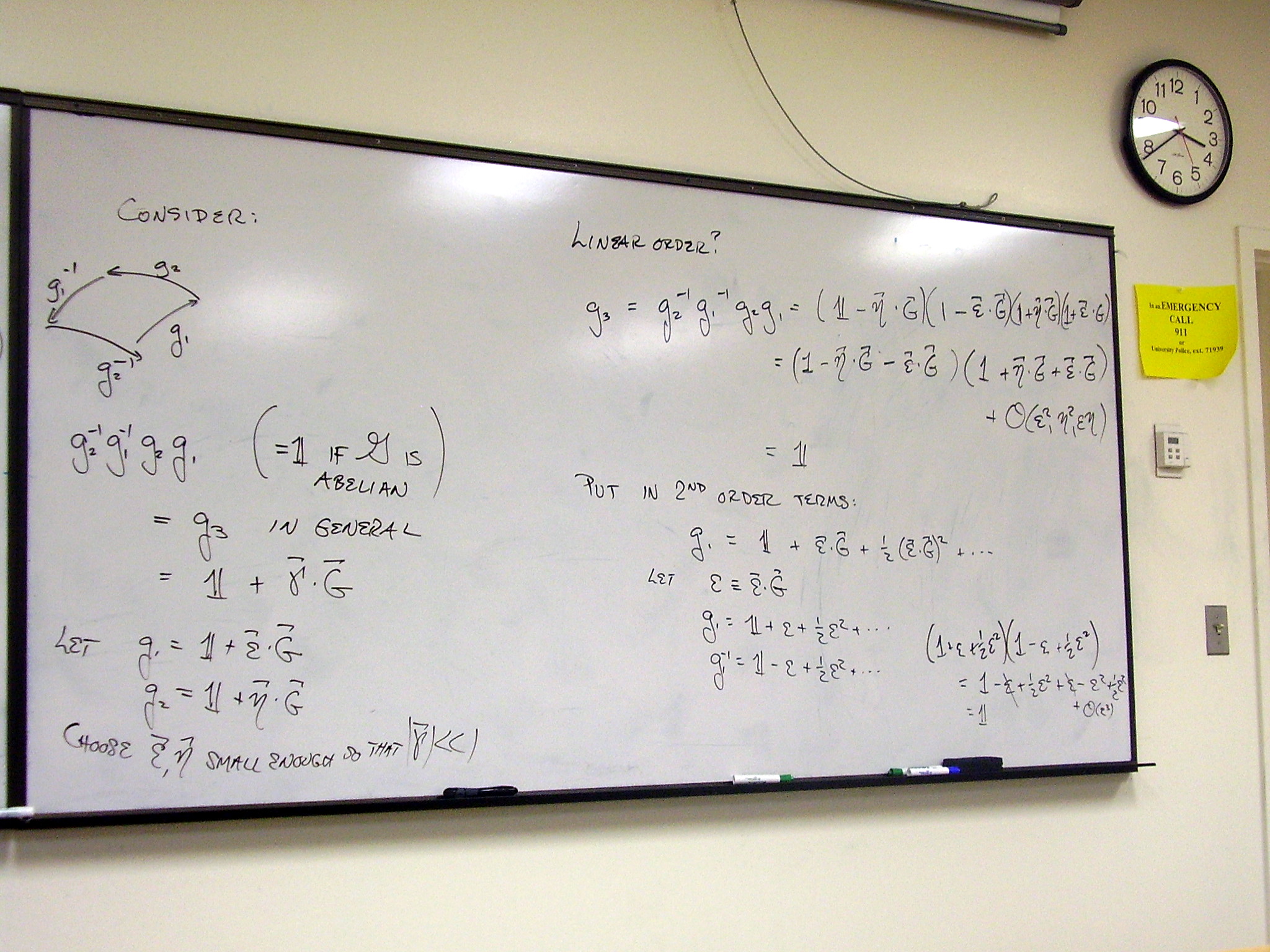
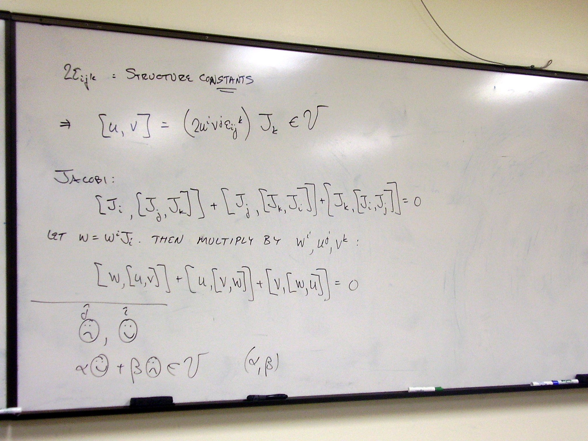
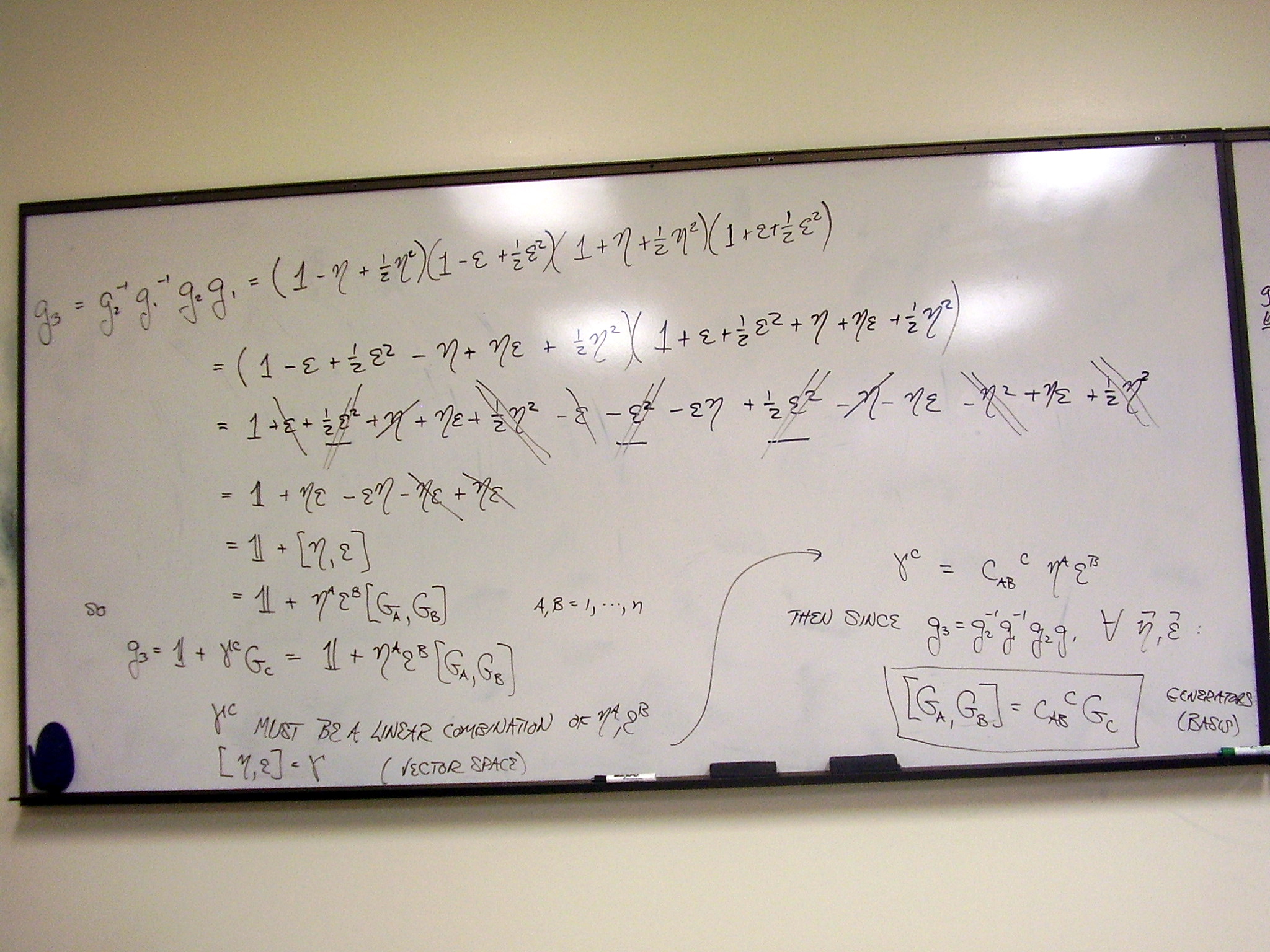
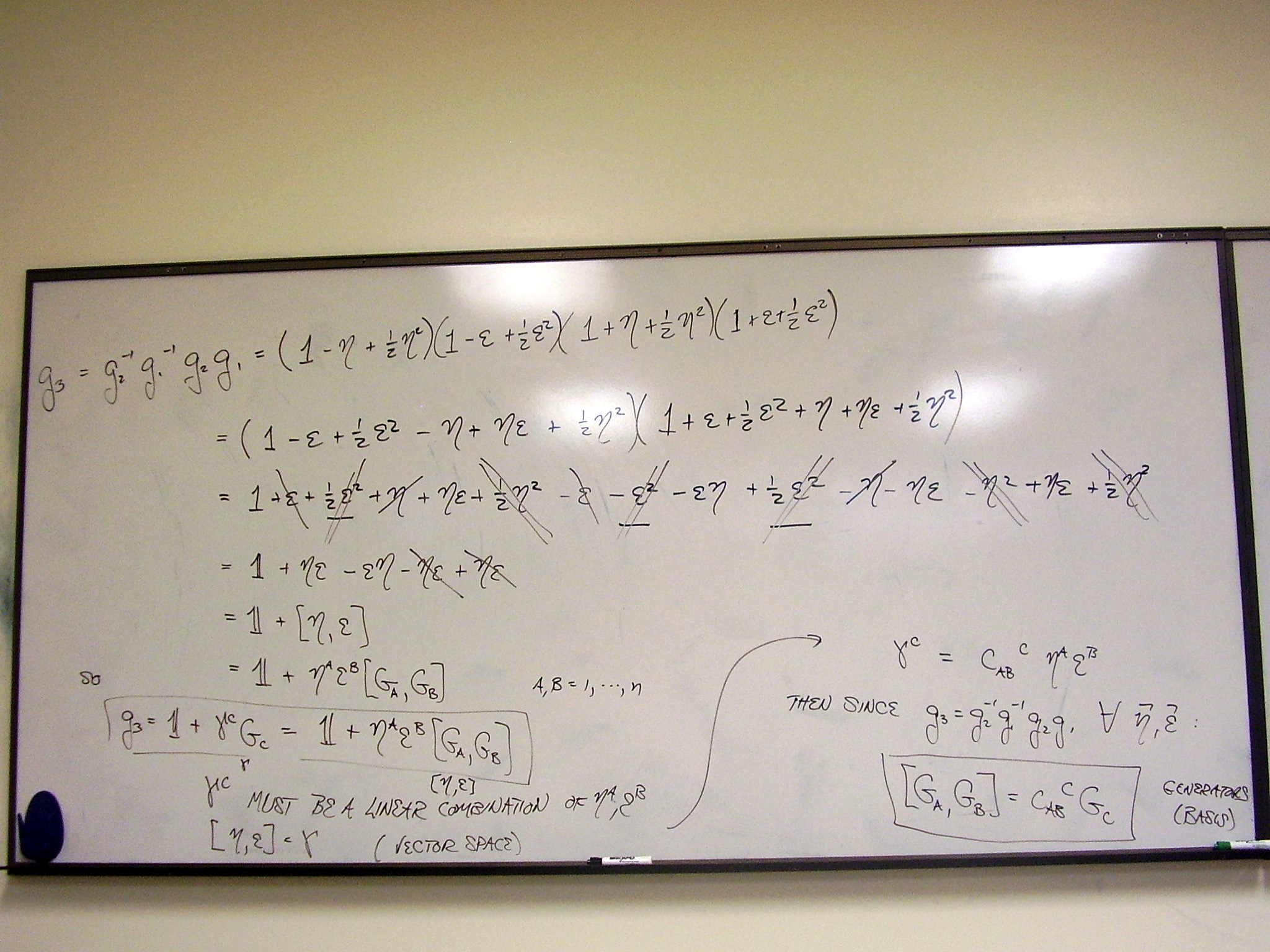
Musing about the Jacobi
identity. We cannot write it using group elements, because there is no addition
in the group – only the group product. However, we can compute the triple
products that are involved in the Jacobi identity:
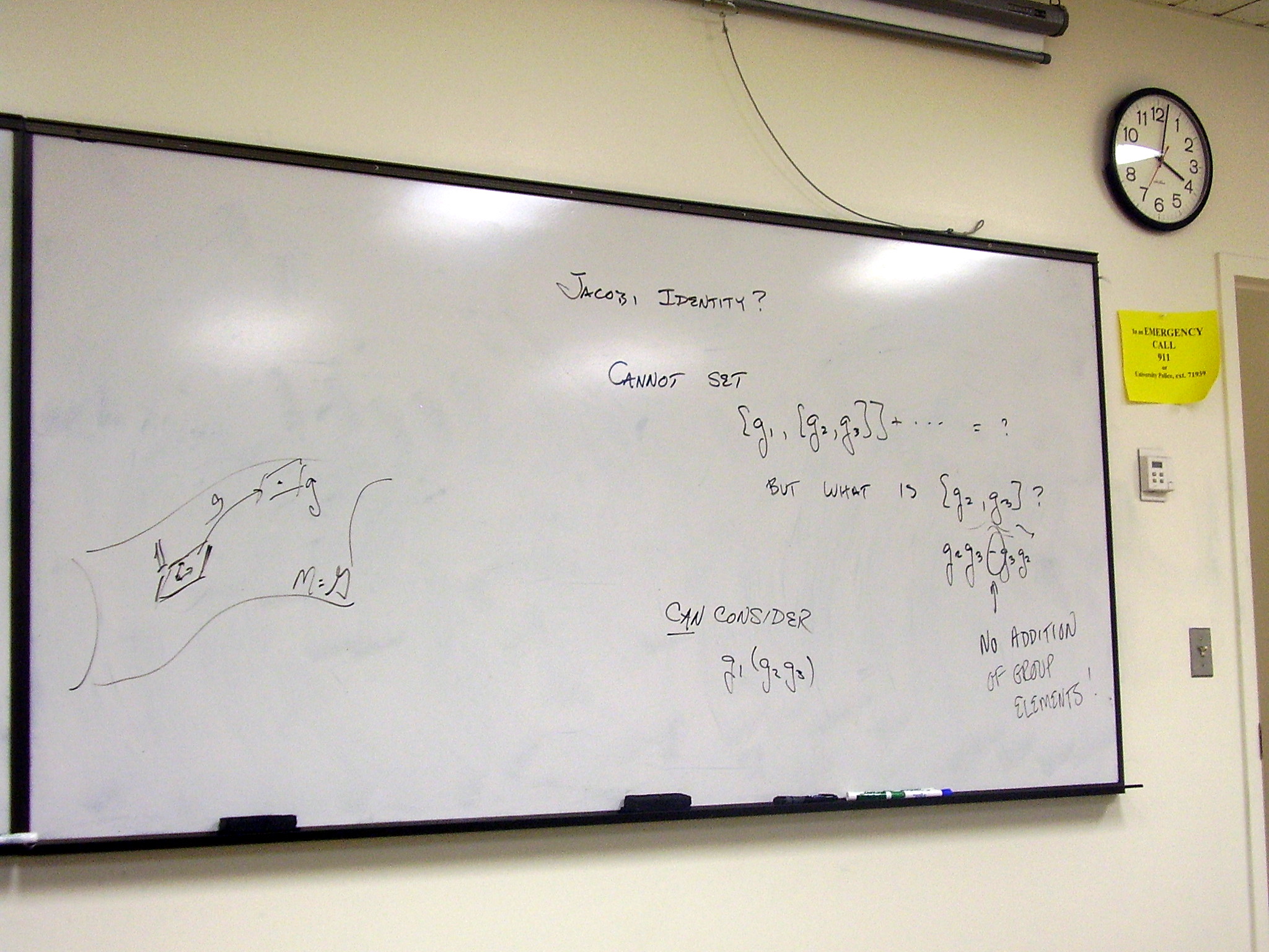
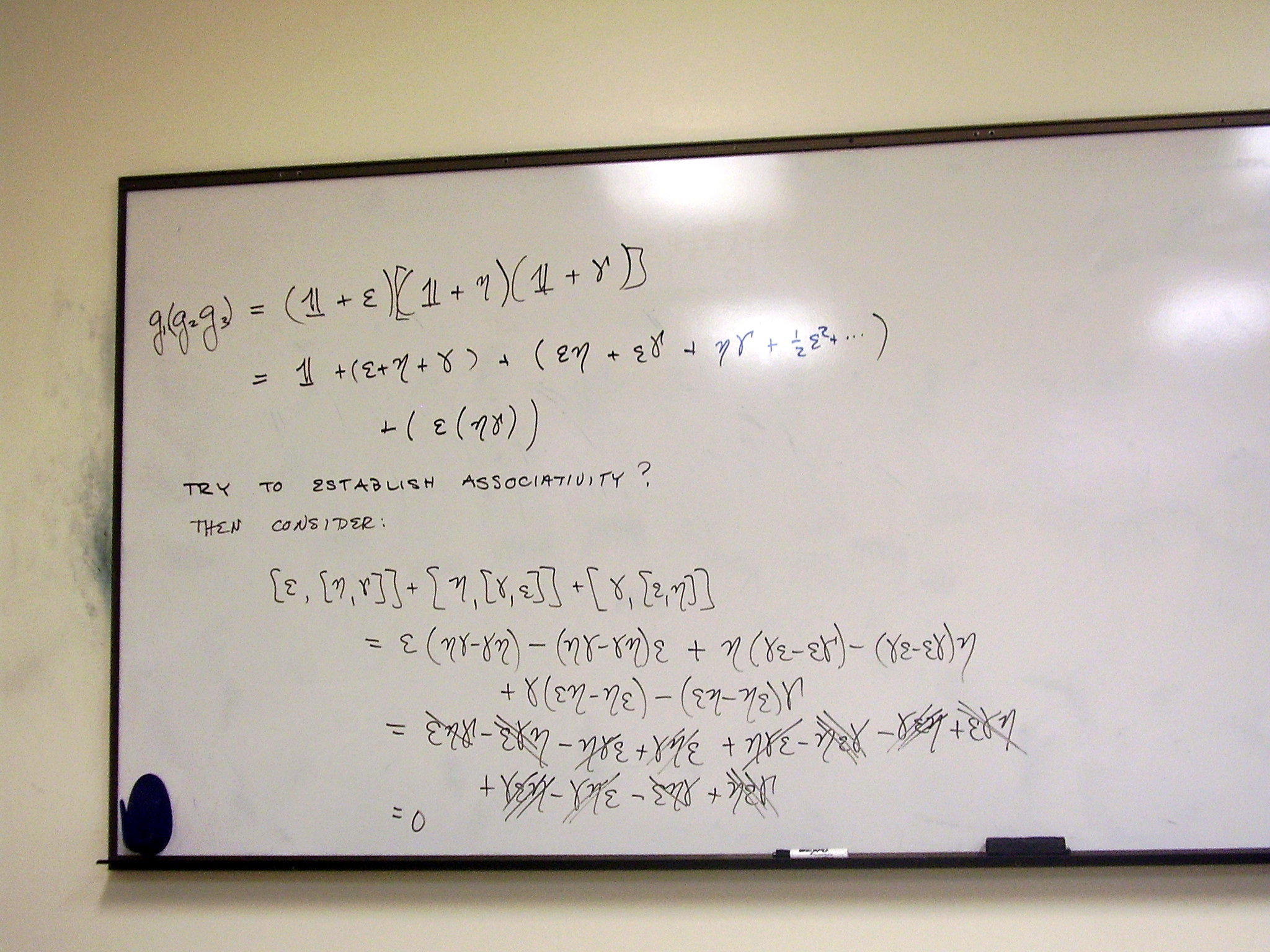
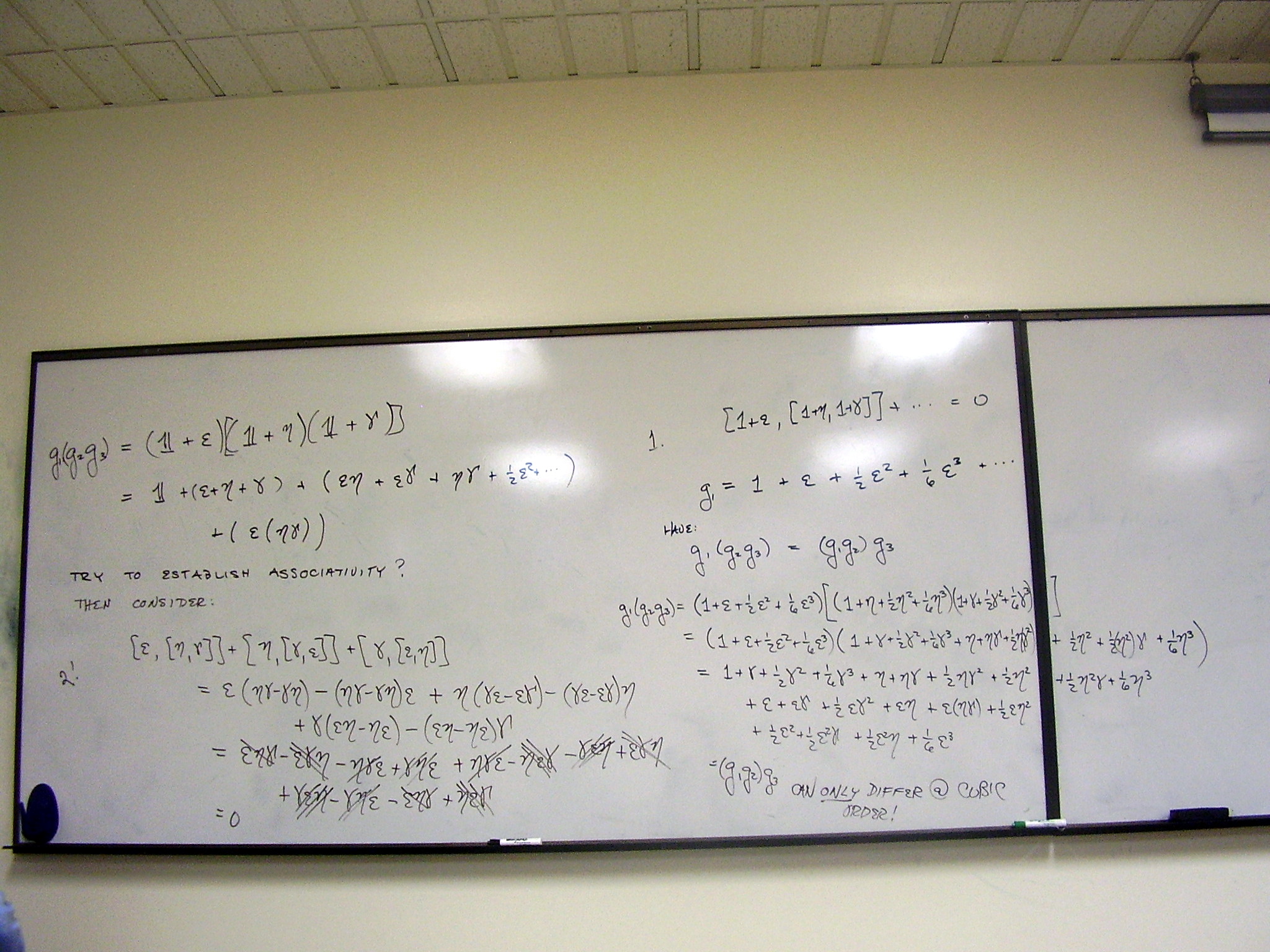
What happens with a triple
product? The cubic order term is simplified if we use associativity. If we
write the Jacobi identity, and multiply out all of the commutators, it is
identically satisfies if the product of generators is associative.
The last slide shows that
the Jacobi identity holds if we can prove that products of generators are
associative. Here’s the proof that the generator product is associative:
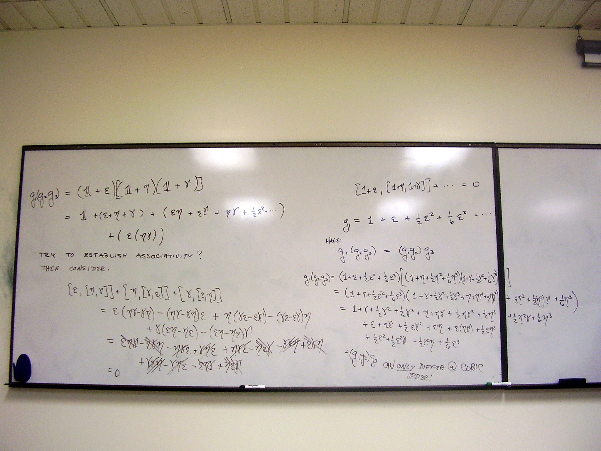
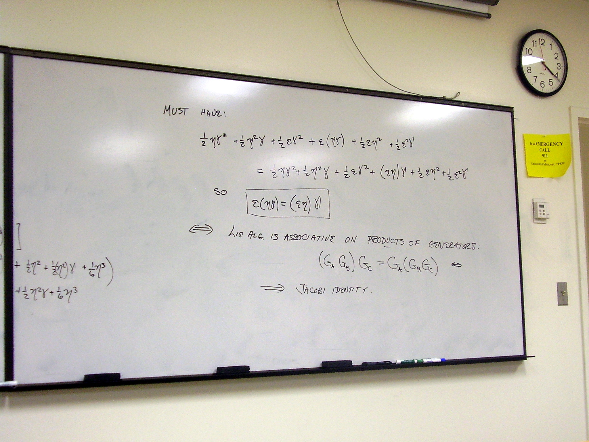
The last two slides again,
after subsequent questions and discussion:
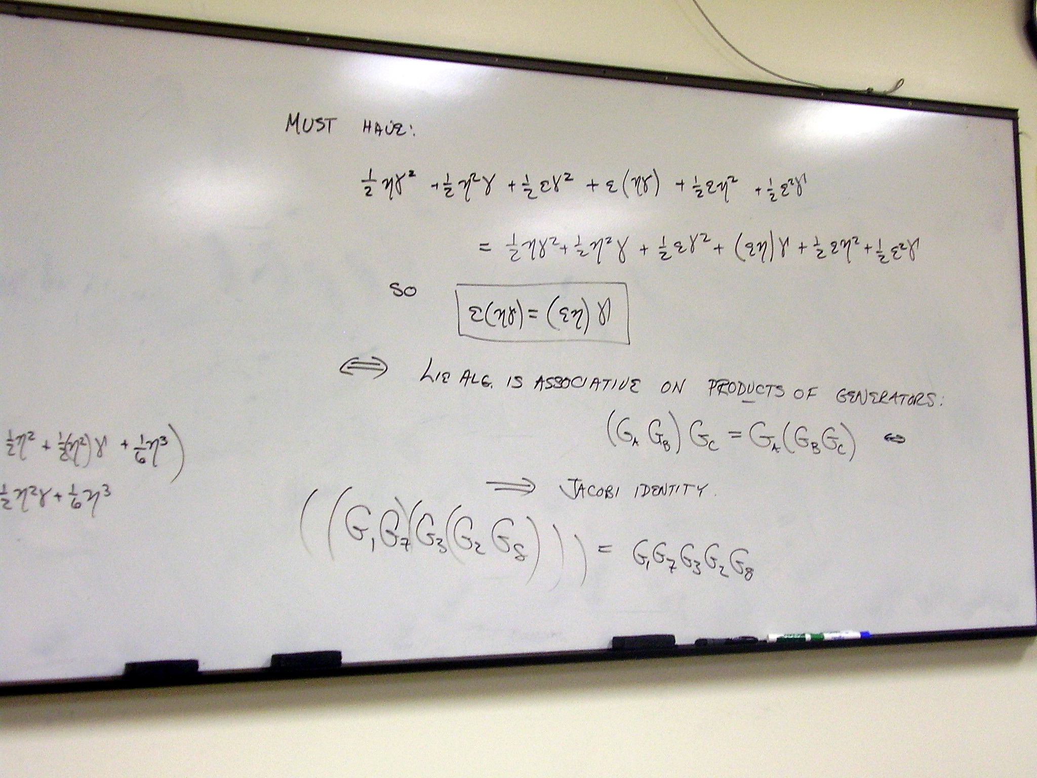
Wednesday, February 4,
2009
Lecture:
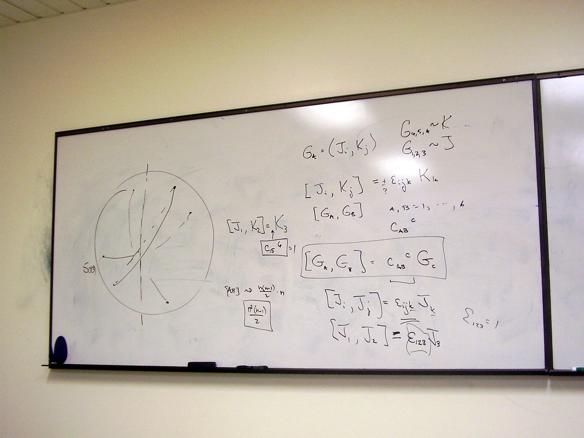
Group quotients; cosets; SO(3)/SO(2)
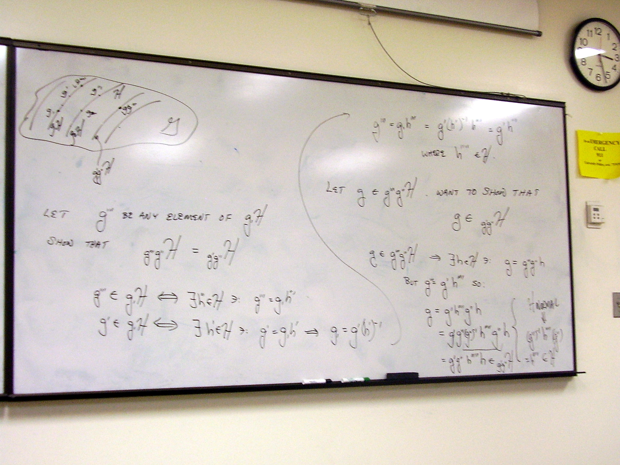
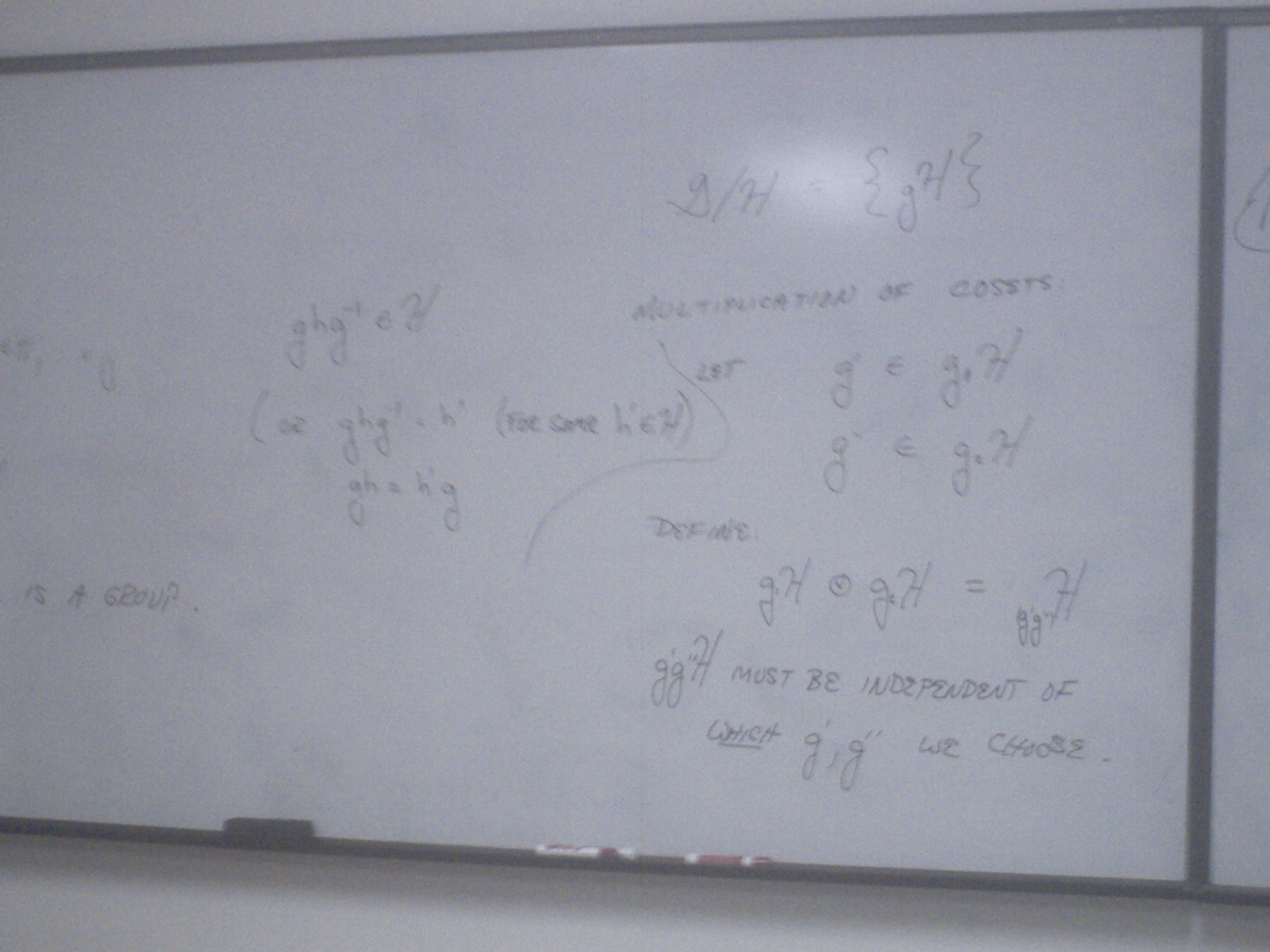
The definition of cosets;
the definition of group quotient:
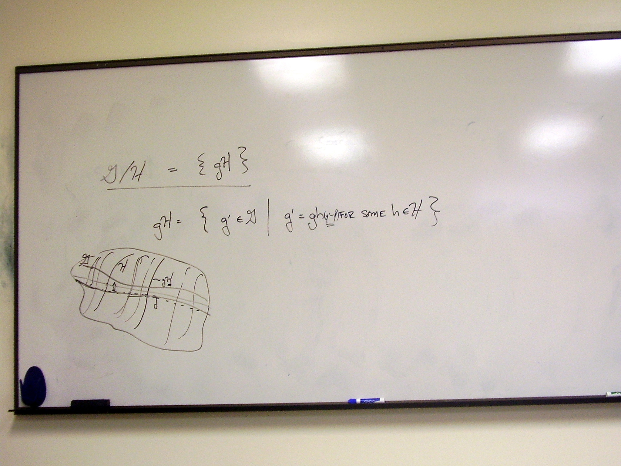
Some overview. Three
quotients we will discuss. Definition of cosets. The group quotient is the
collection of all cosets.
Example: Describe a coset of SO(3)/SO(2).
Picking a coset (3 similar slides; slight changes/additions in each)
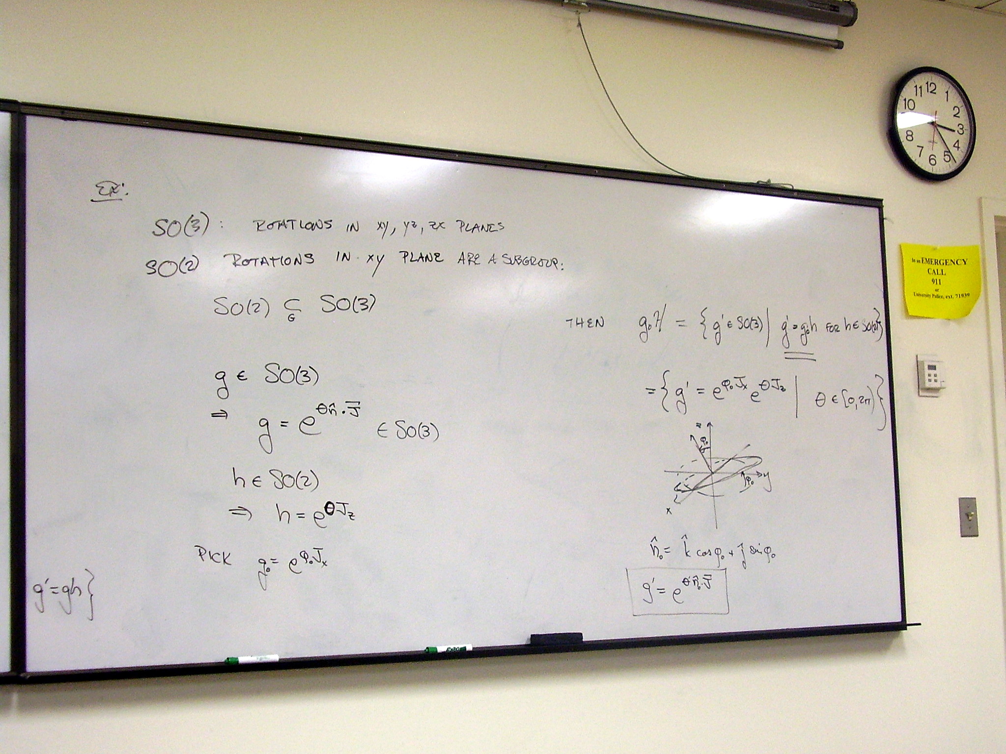
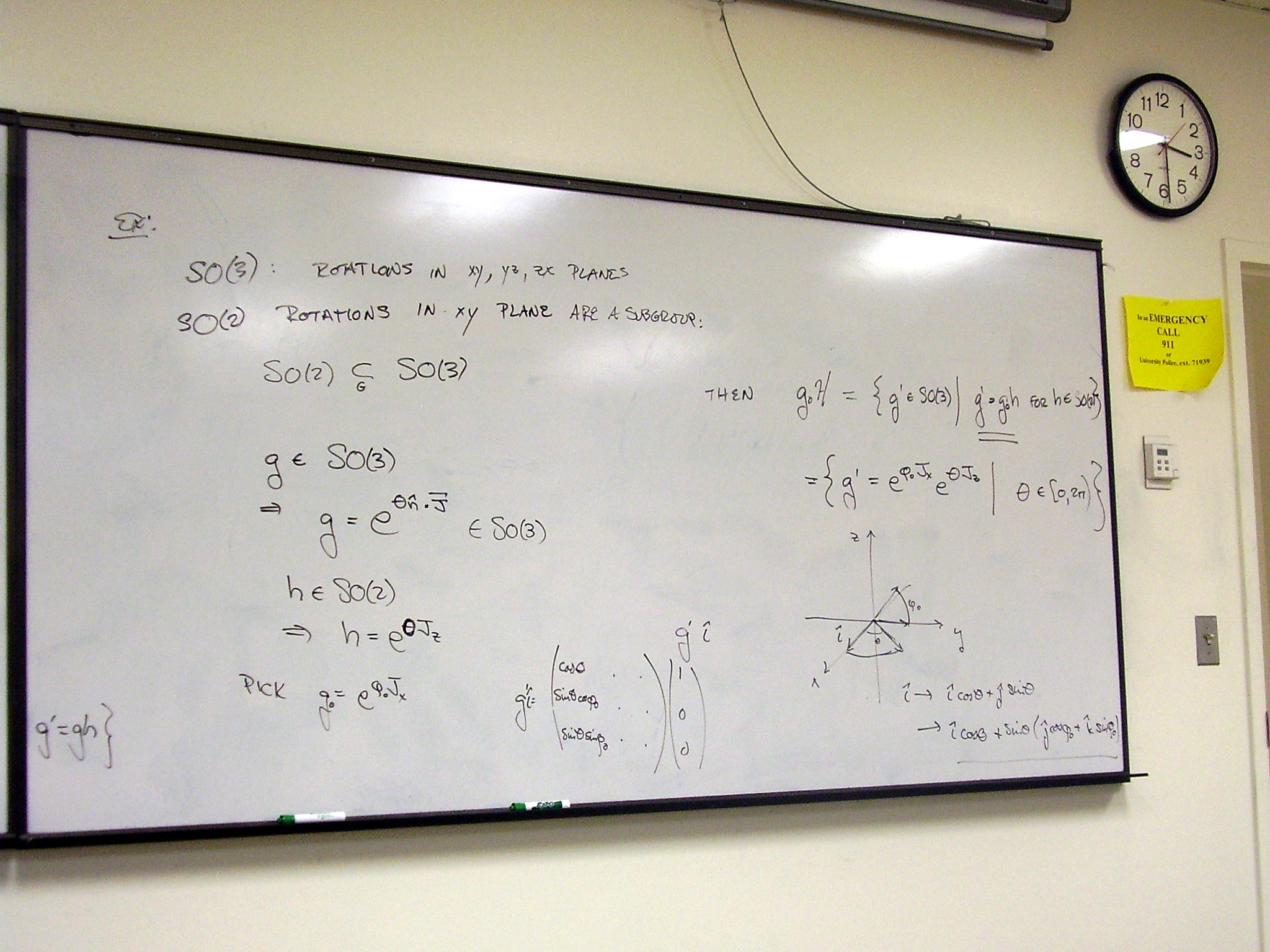
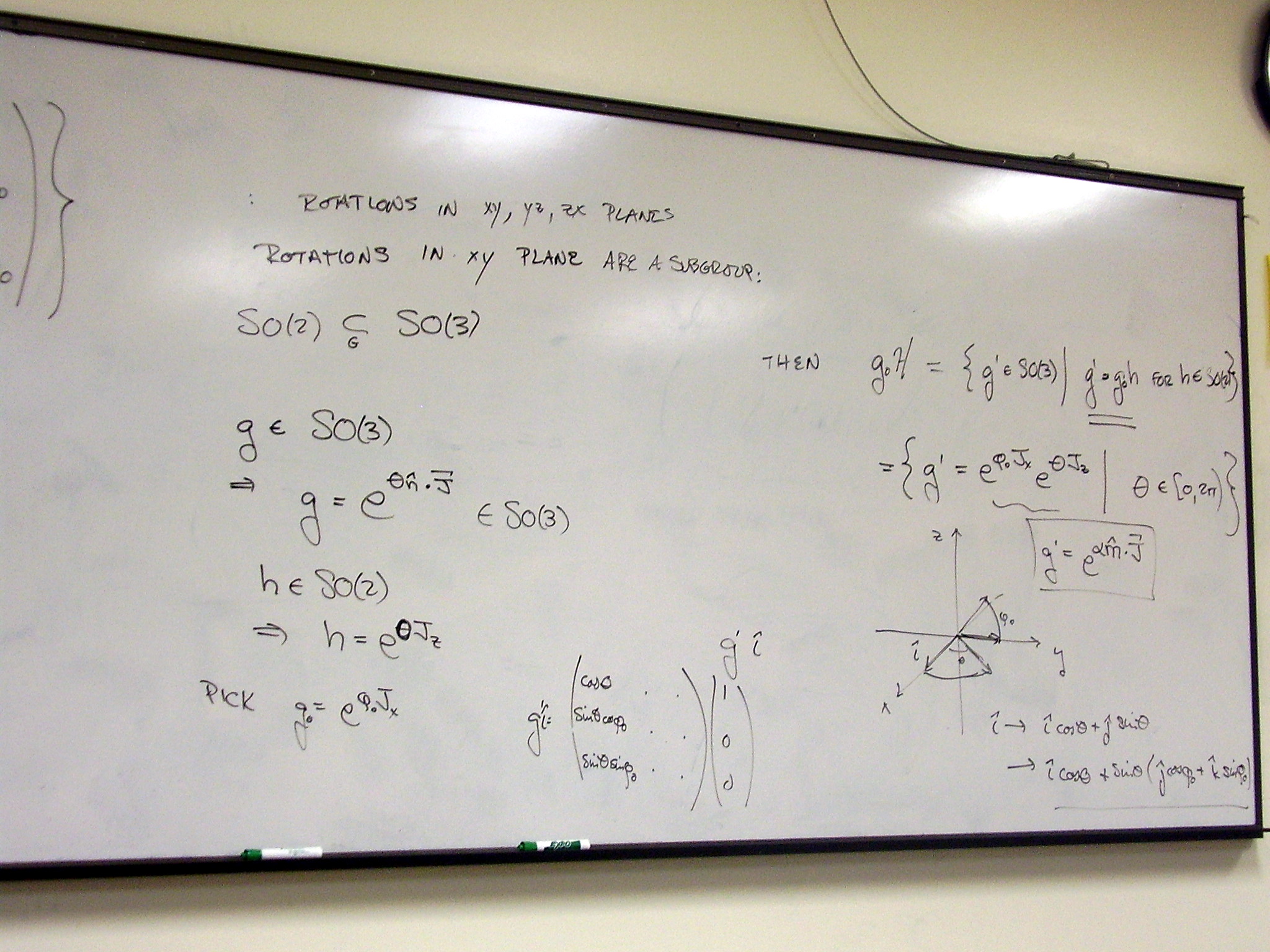
Find the set of
transformation matrices by checking the effect of a general element of the
coset on unit vectors.
Check that the matrix we
find is a rotation, i.e., that its transpose is its inverse.
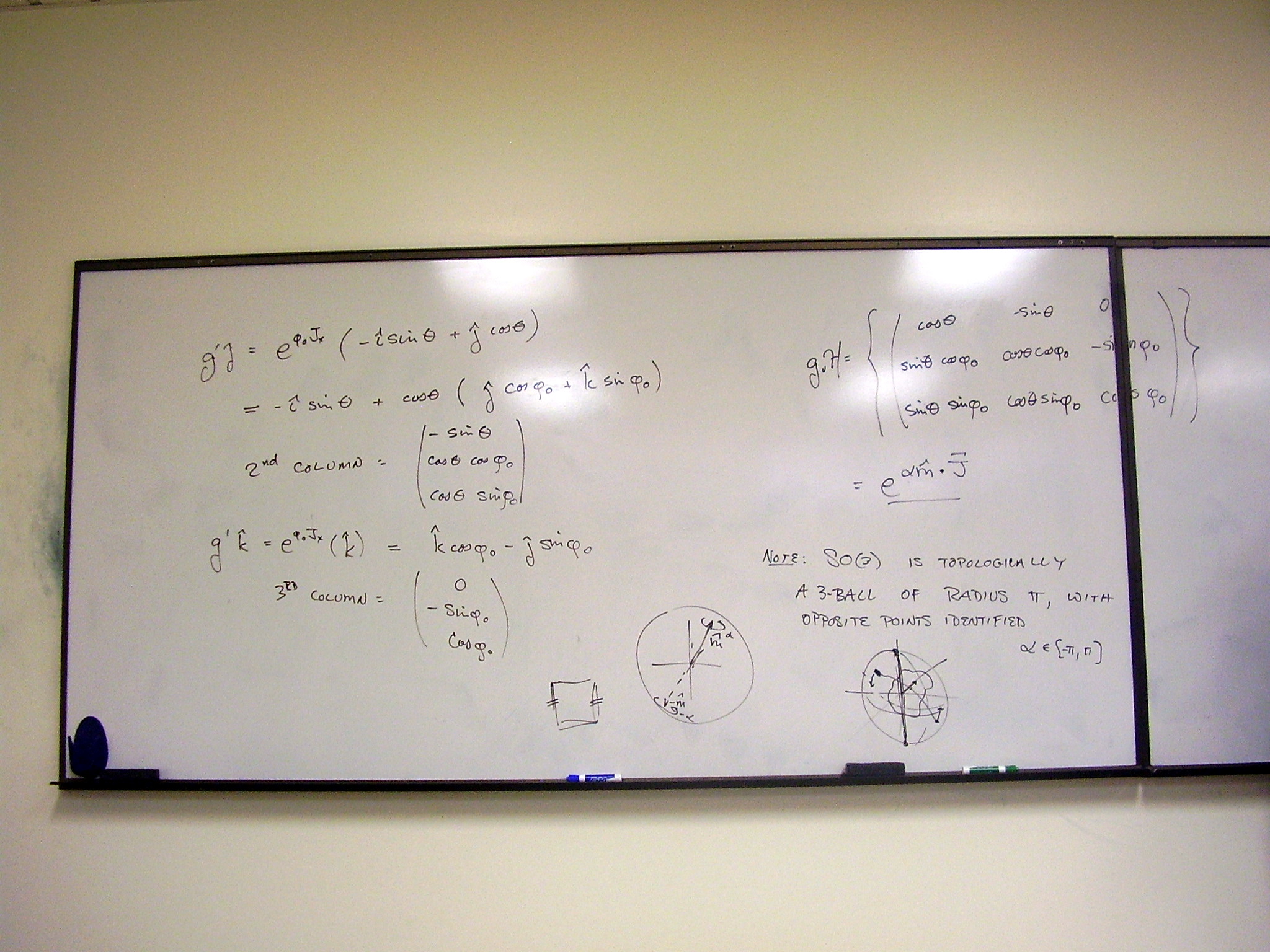
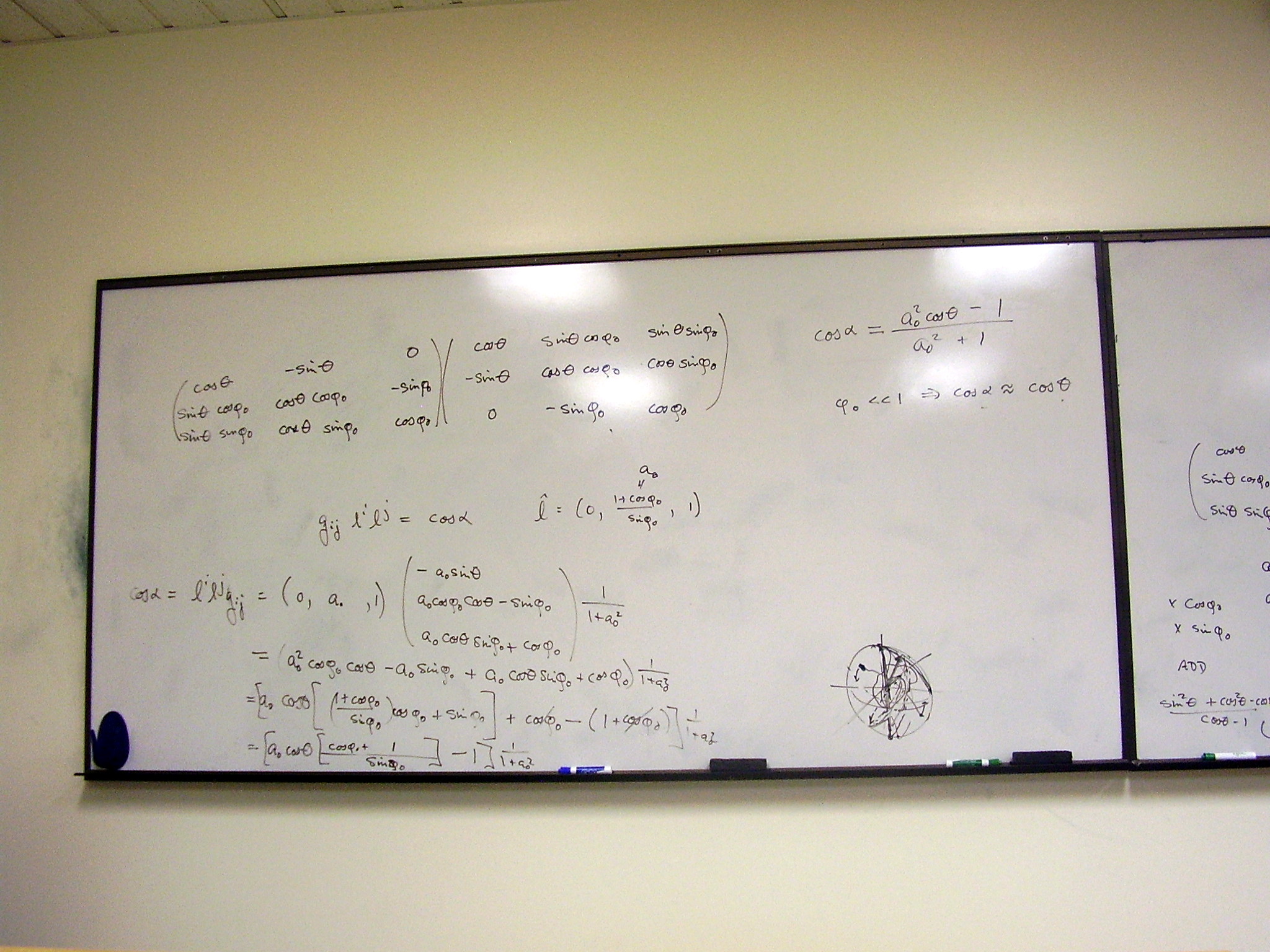
Find the axis of rotation.
The transformation will leave the axis unchanged, so it will be an eigenvector
with eigenvalue 1. Normalize the axis vector. Find a vector l which is
orthogonal to the axis of rotation for all elements of the coset (3 similar slides).
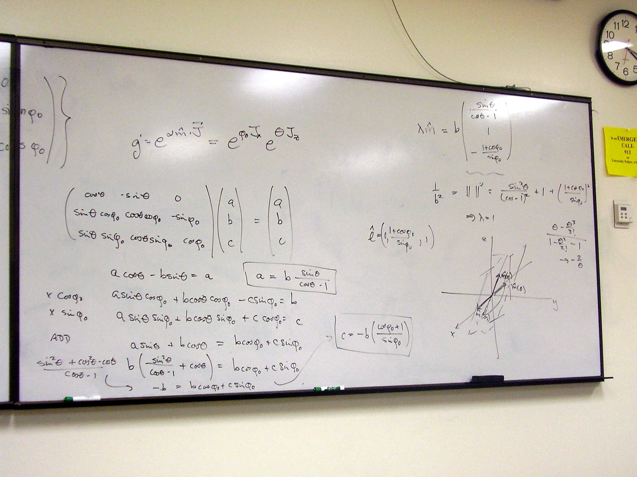
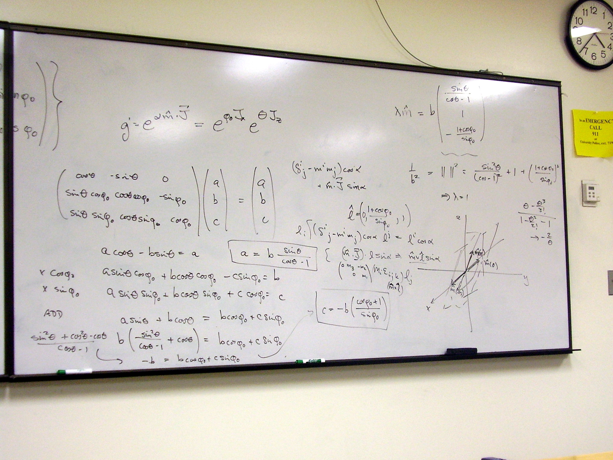
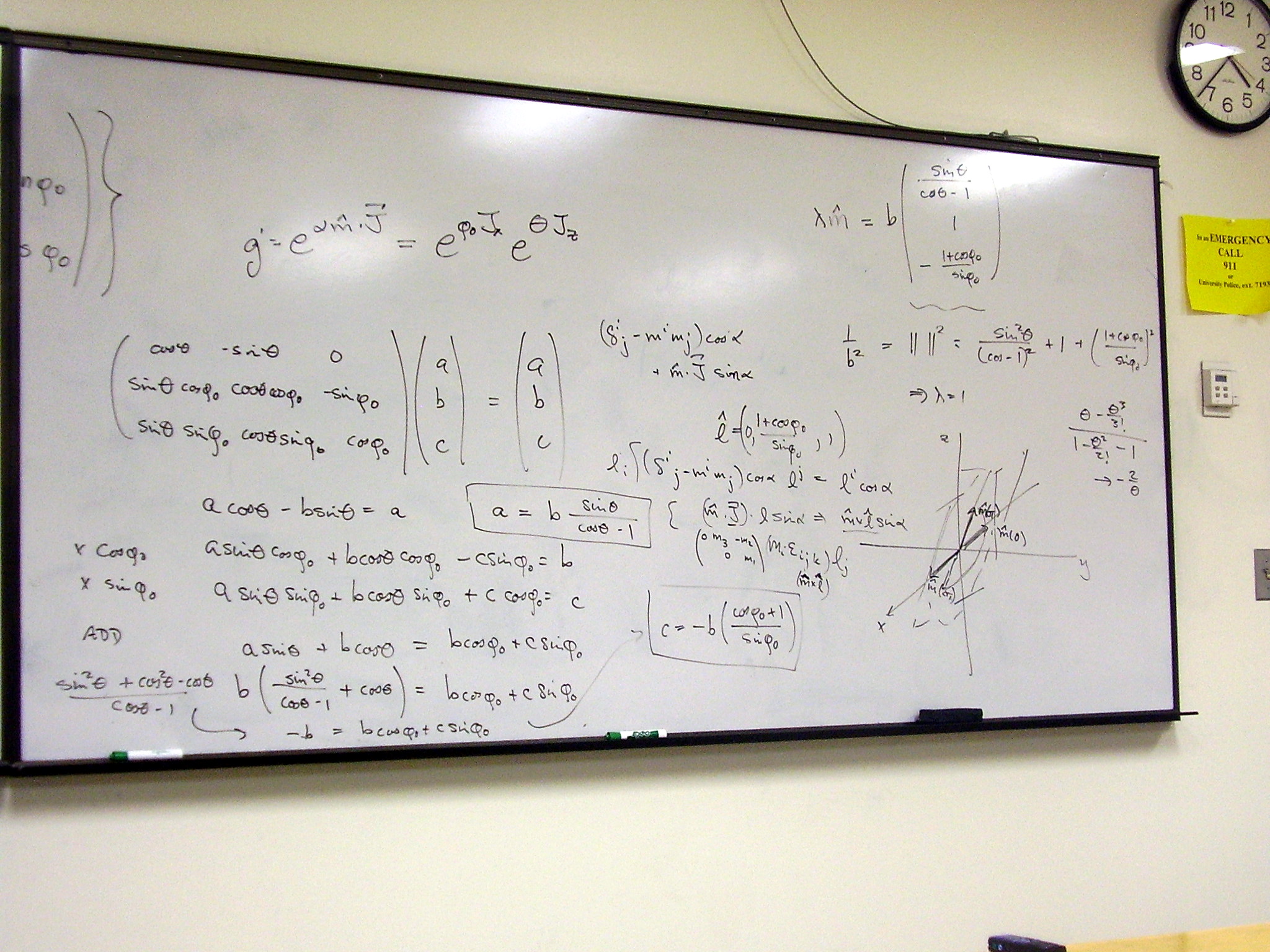
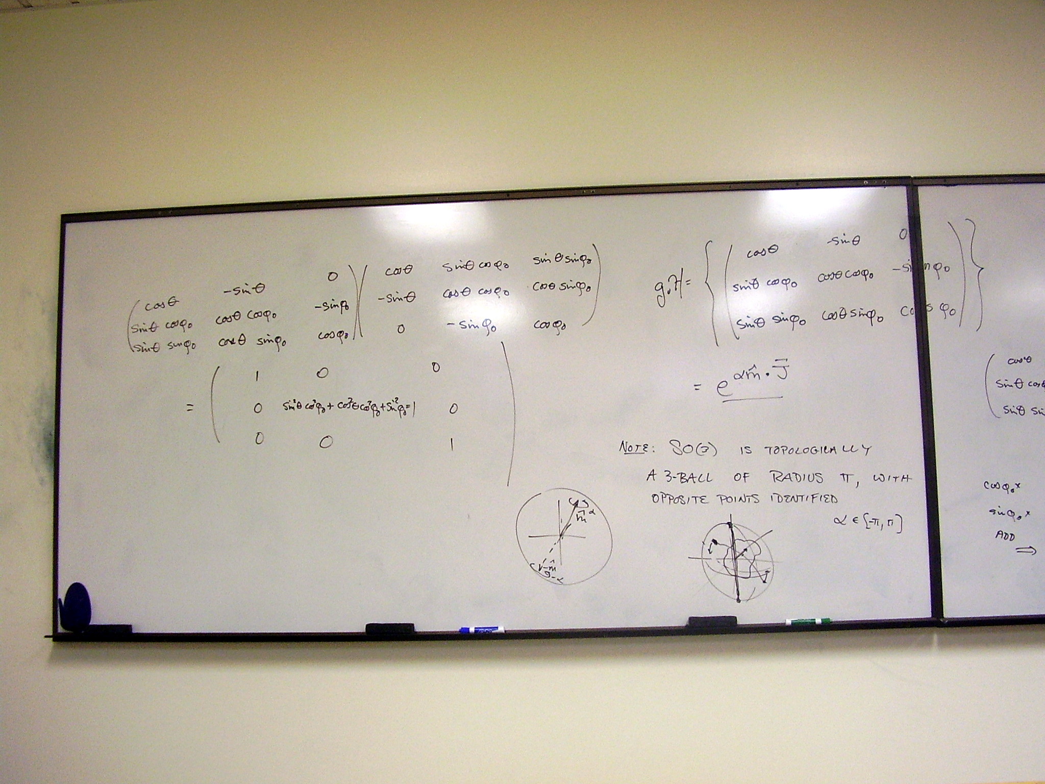
Find the angle of rotation
for each element of the coset. Plot the coset as a curve in SO(3), where the
manifold SO(3) is a 3-dimensional ball of radius π.
A better picture:
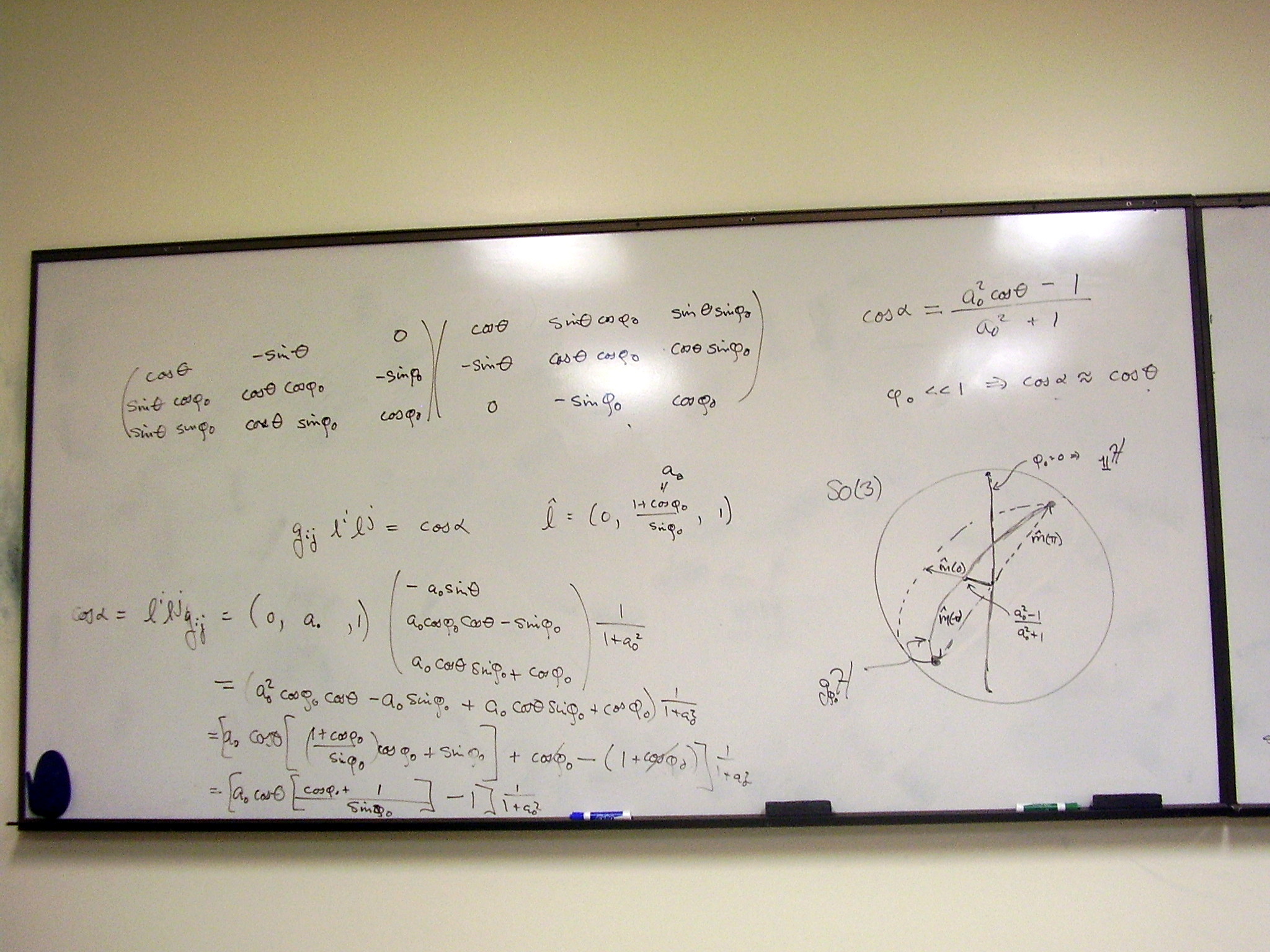
Friday, February 6,
2009
Lecture:
Quotients and cosets. Examples: SO(3) and SO(2); O(3) and SO(3)
Calculation of the general form
of a rotation using SO(3). Includes a correction of the previous calculation:
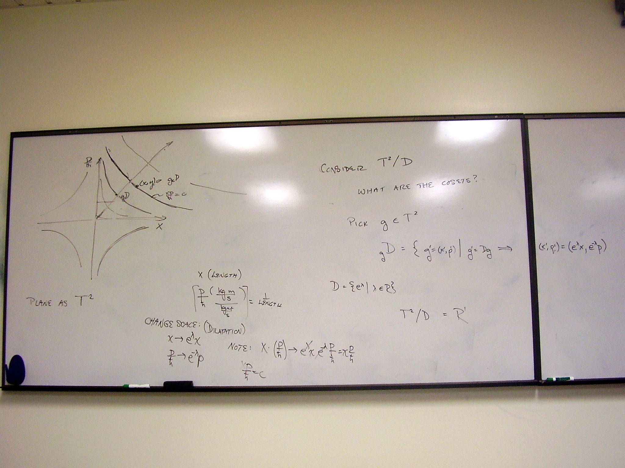
A simple example of a coset,
using dilatations as a subset of the phase space plane. This is not a group
quotient, because phase space dilatations (which stretch p while contracting x,
and vice versa, thereby tracing curves xp = c) are not a subgroup of the
translation group of the plane. We can construct a group spanning the phase space
plane and including dilatations by adding the hyperbolas orthogonal to the path
of the dilatations, p2 - x2 = c. However, the generators of these two sets of hyperbolas
don’t commute: instead we find a third generator, which gives circles in the xp
plane. The 3-dimensional Lie group we have built up is SL(2). The quotient by
the dilatations is complicated.
A coset of SO(2) as a
subgroup of SO(3). We worked this out at the end of the previous lecture, but
this is a better picture:
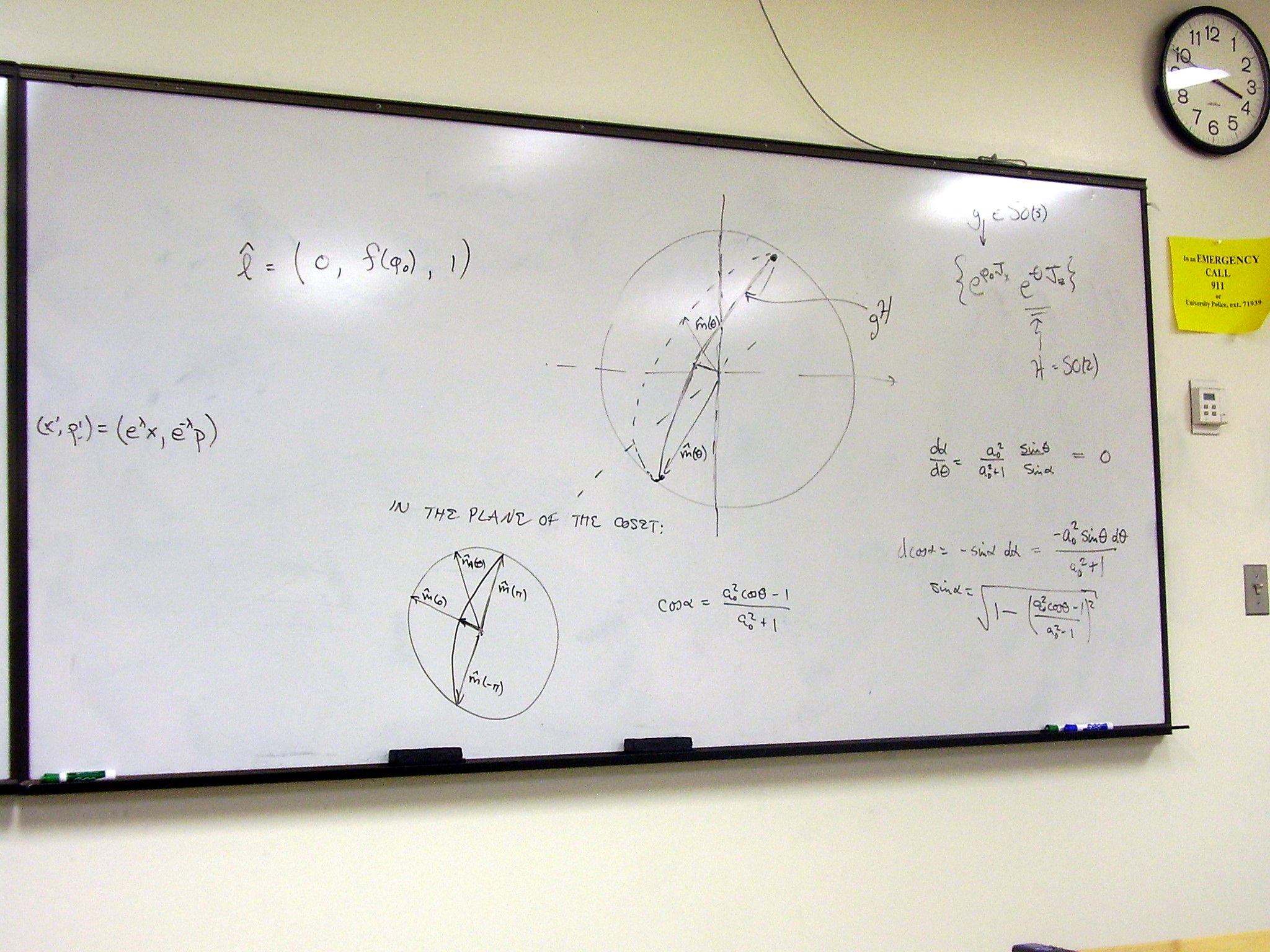
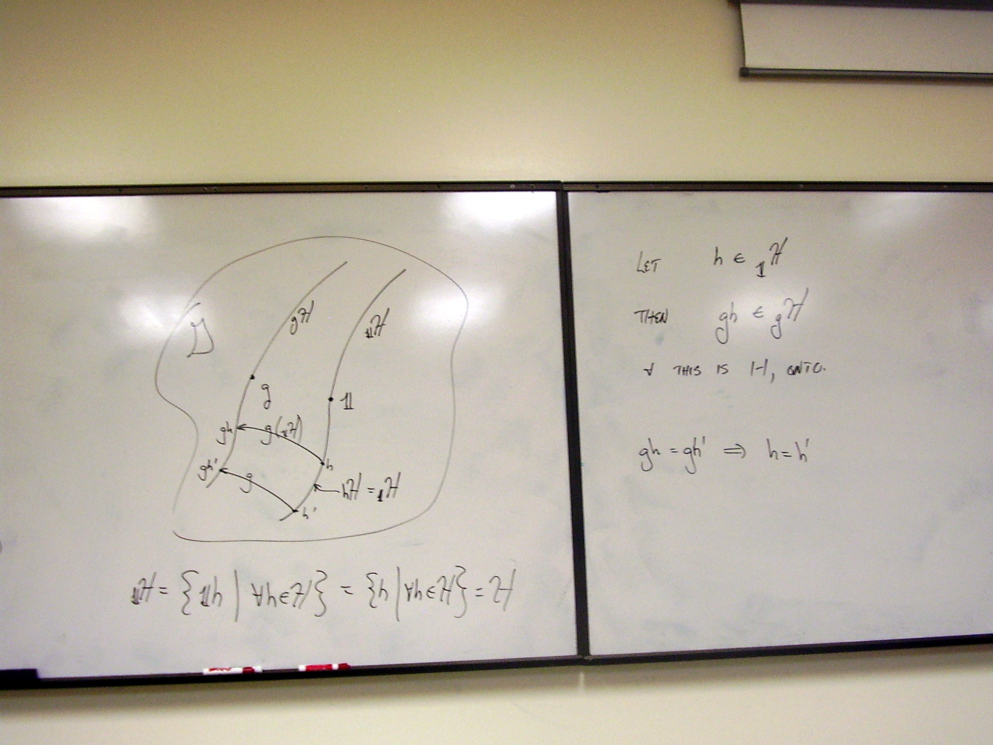
Theorem: If two cosets
intersect, then they coincide. The proof.
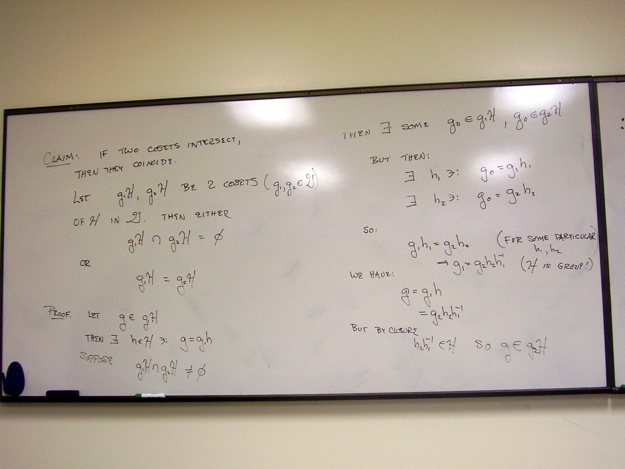
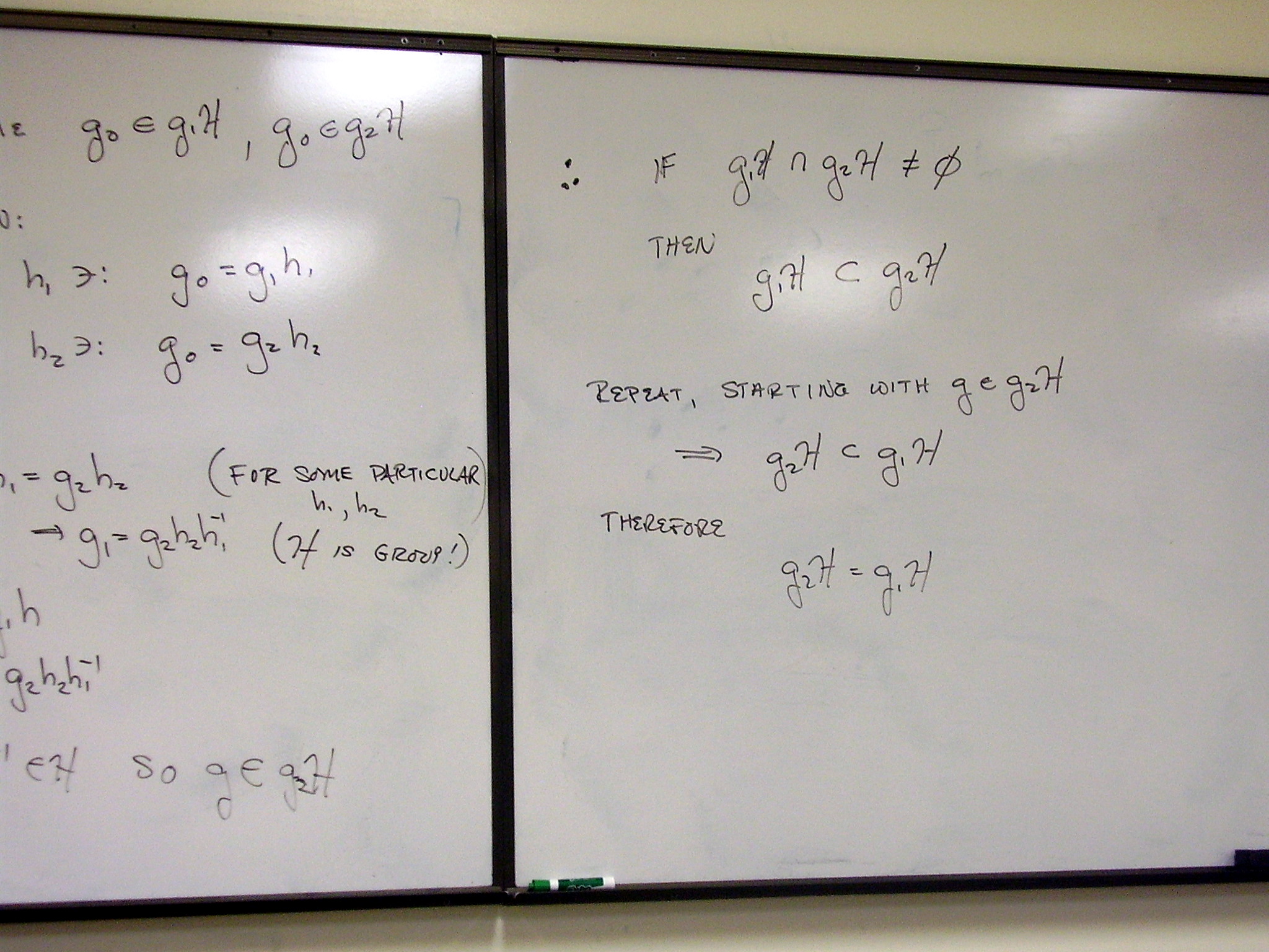
Theorem: Each element of a
Lie group lies in exactly one coset. The proof is immediate:
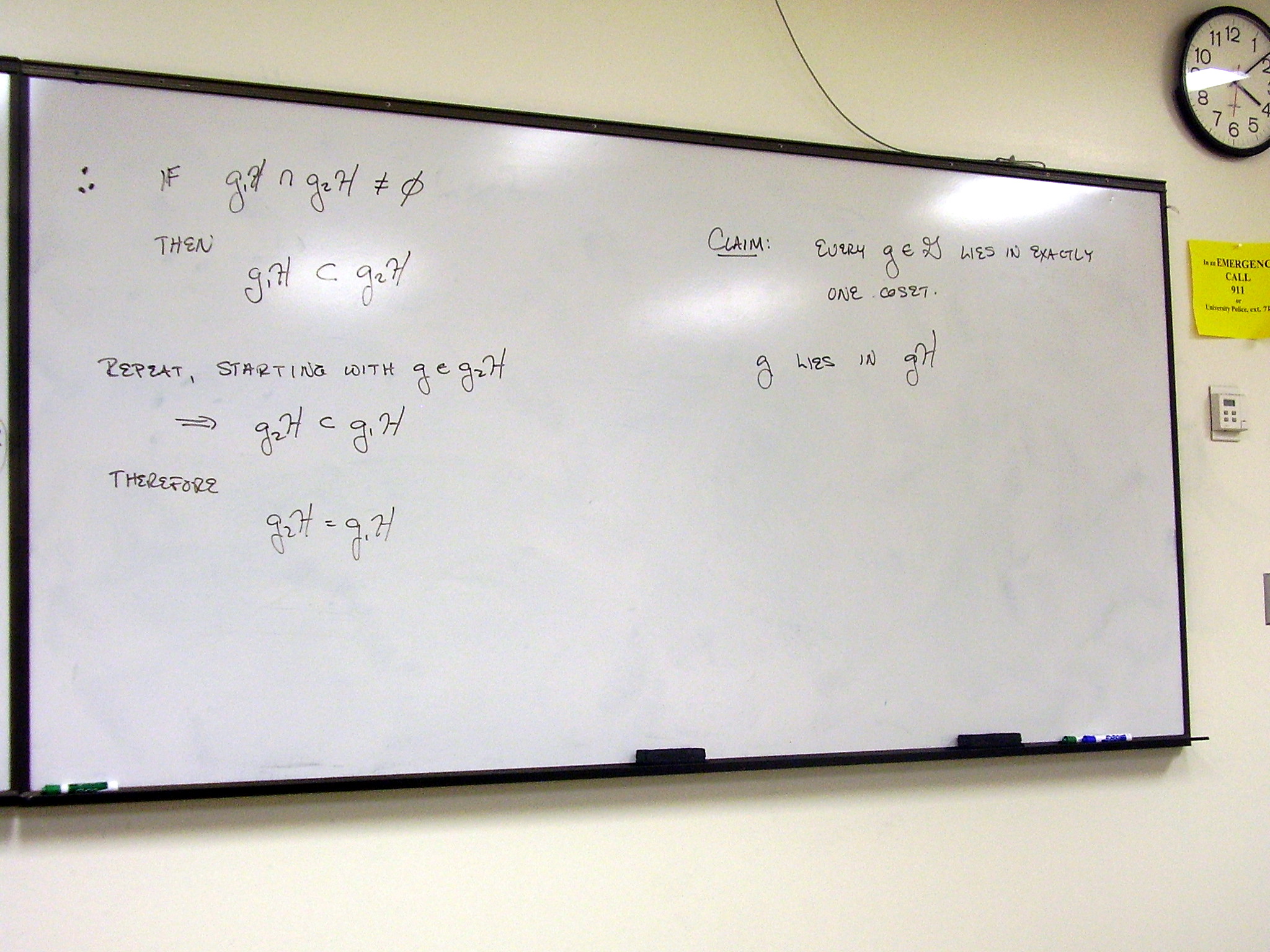
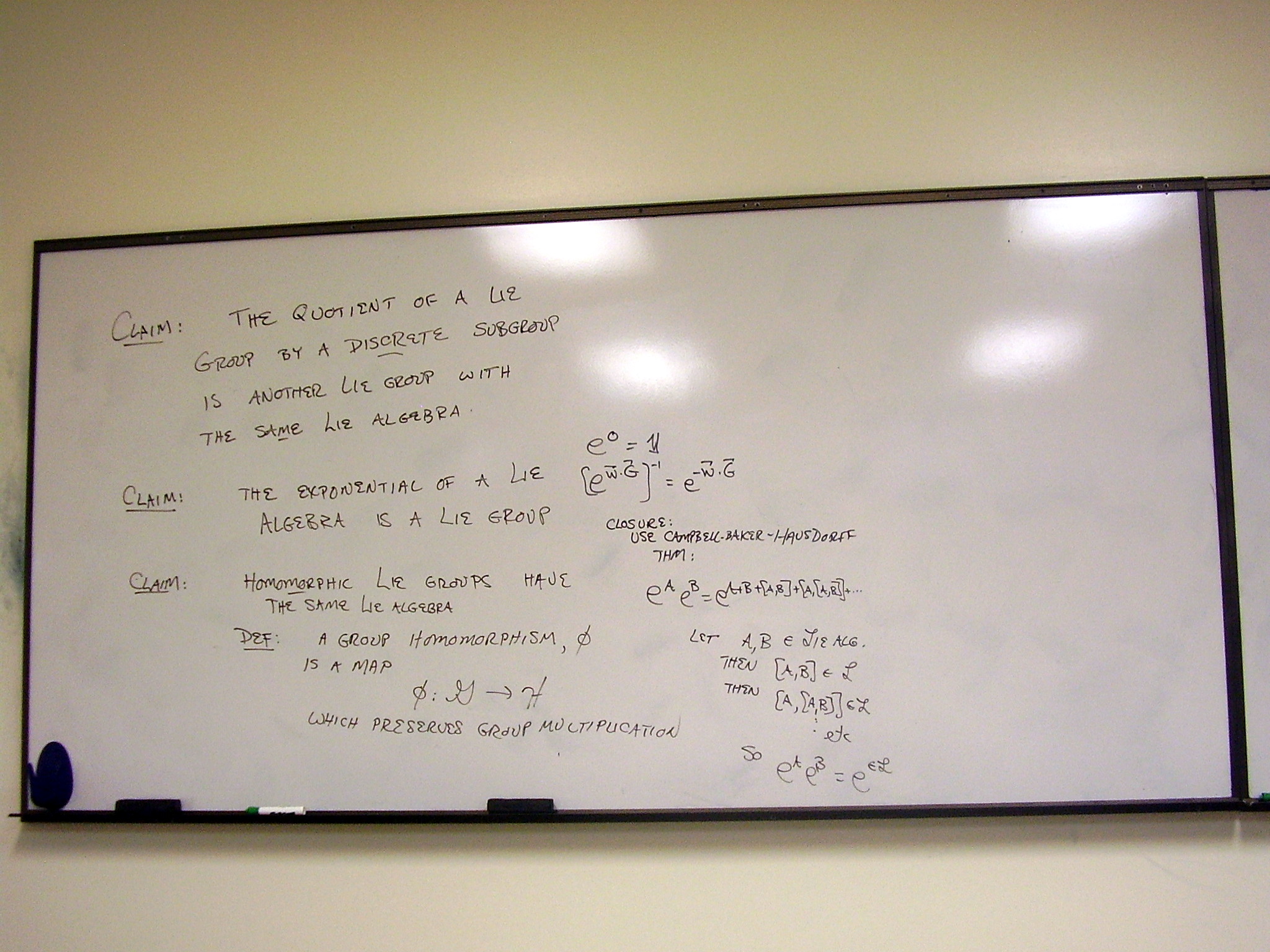
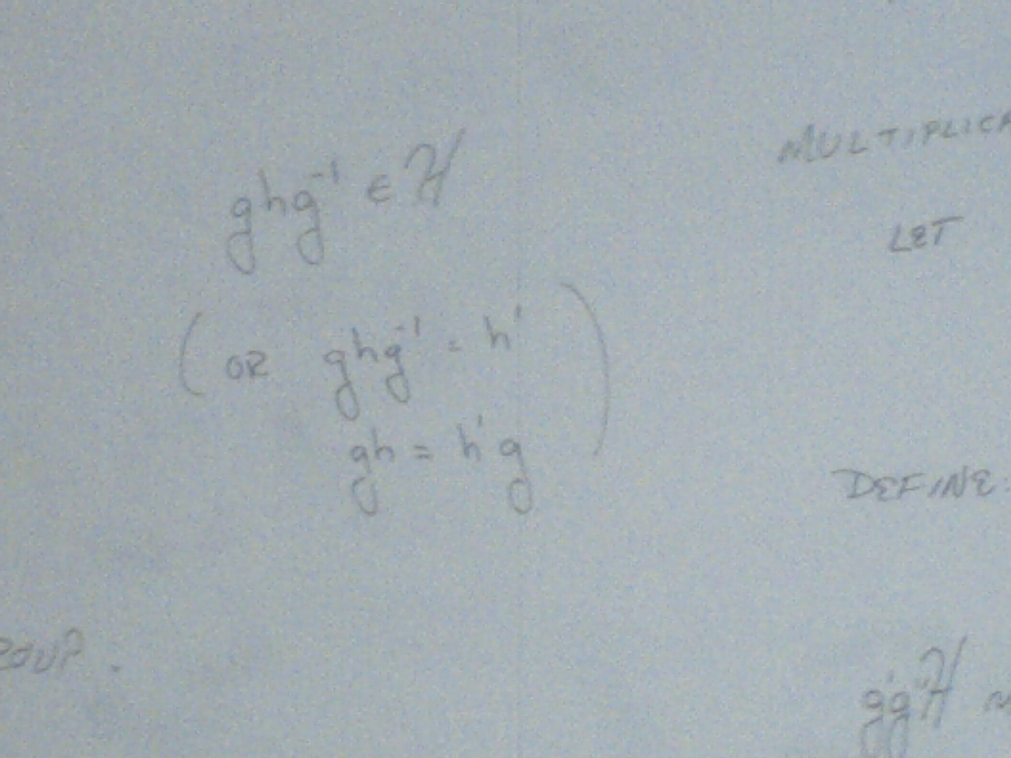
Some claims and
definitions. Group homomorphism.
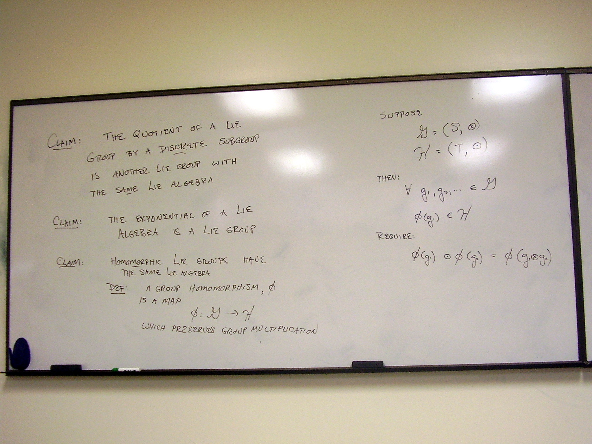
Three-quarters of the
proof that the exponential of a Lie algebra is a Lie group (closure, identity
and inverse follow easily from the Campbell-Baker-Hausdorff theorem):
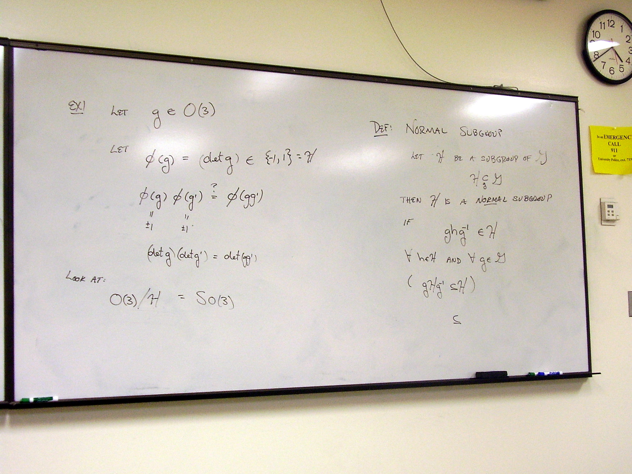
An example – the
quotient of O(3) by the two element group Z2 = {1, -1 under
multiplication} sets up an equivalence relation between rotations with
determinant +1 and -1. The quotient O(3)/Z2 then gives SO(3). Also, the definition of a normal
subgroup.
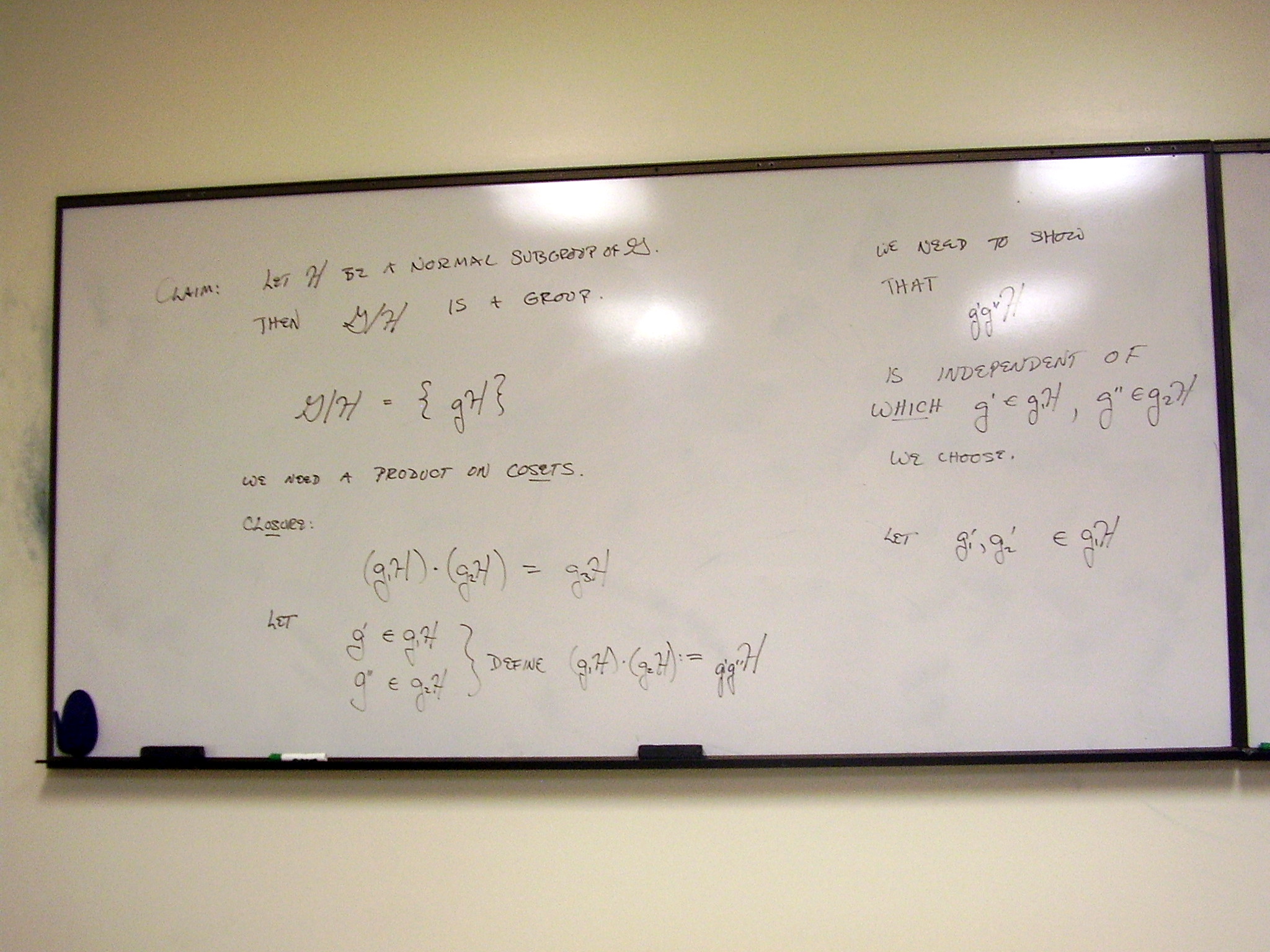
Theorem: The quotient of a
group by a normal subgroup is a group. We’ll do the proof next week.
Monday, February 9,
2009
Lecture:
Quotient by a discrete subgroup.
Example: SU(2) and SO(3)
Theorem on quotients by
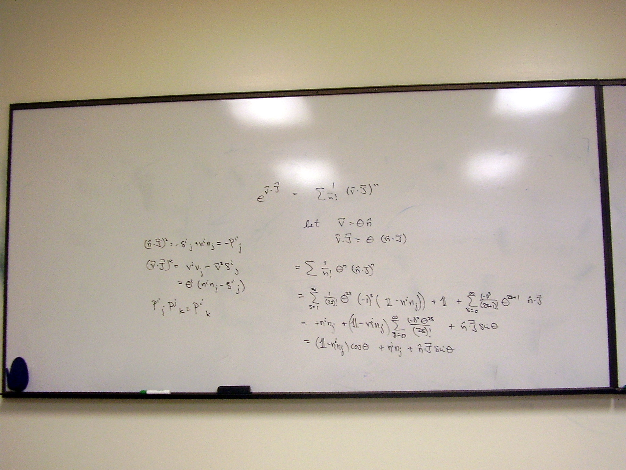
discrete subgroups. The Lie algebra of SO(3). Beginning of SU(2):
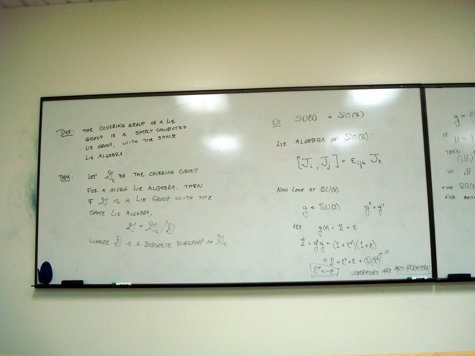
Finding the generators and
Lie algebra of SU(2):
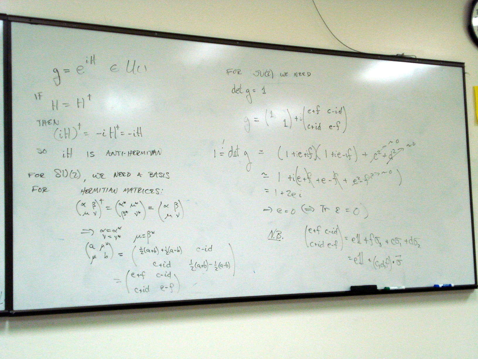
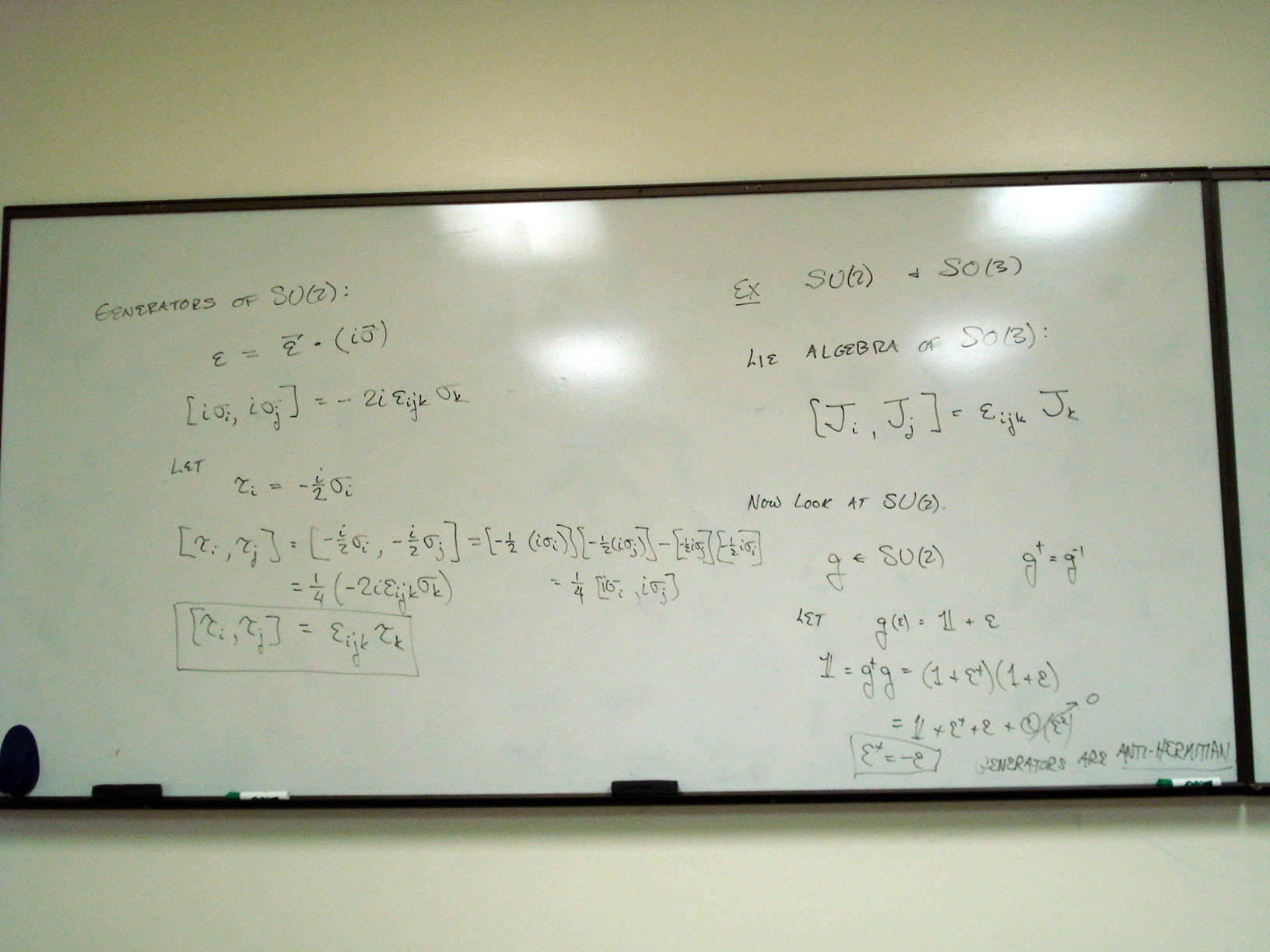
Lie algebra of SU(2). Action
of SU(2) on a 3-vector:
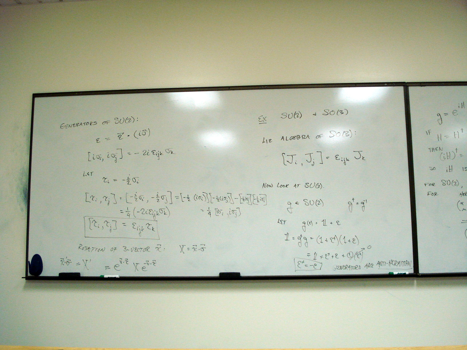
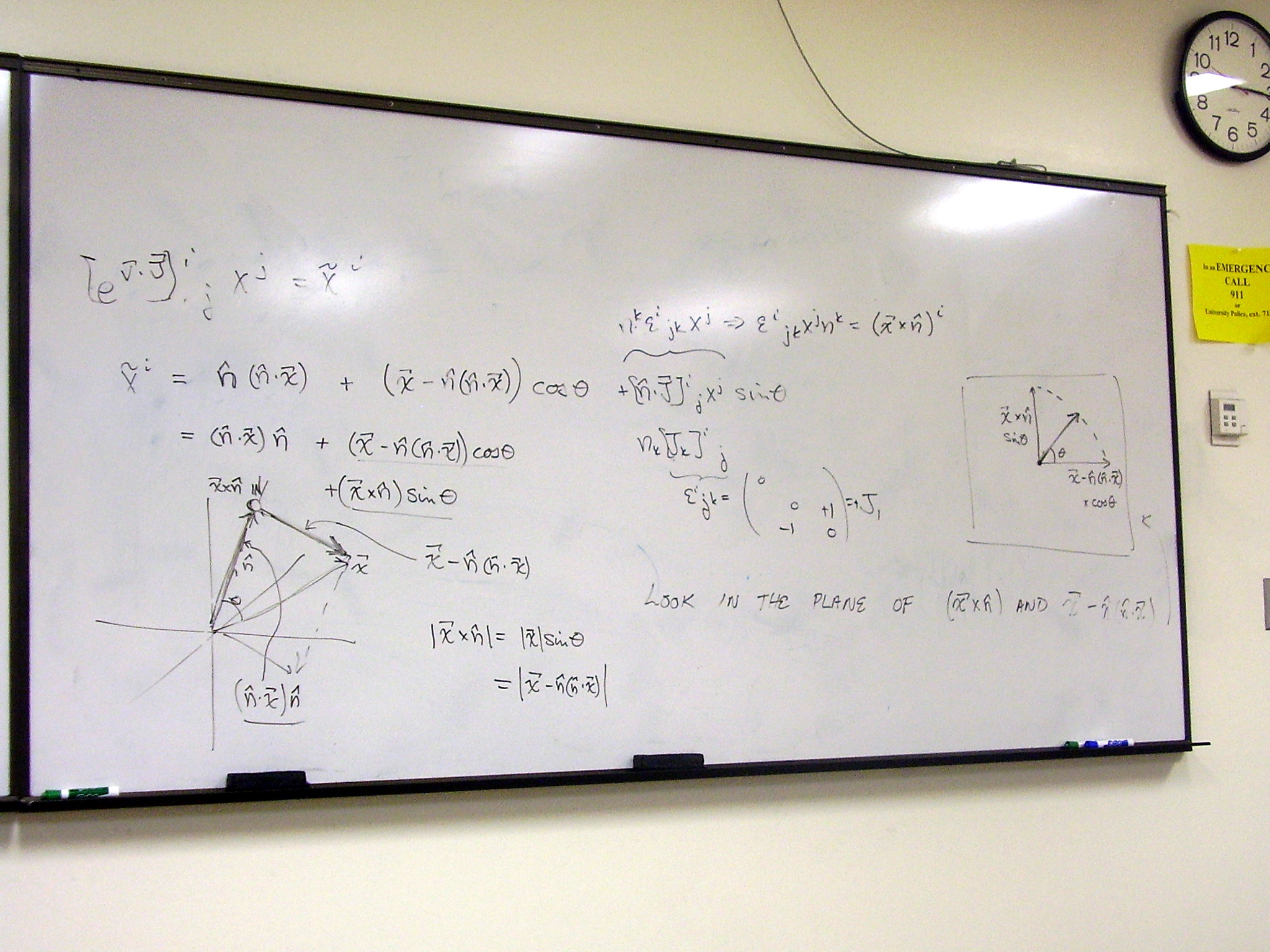
Proving the 2:1 cover by
SU(2) of SO(3). For every rotation of a real 3-vector, x, there are exactly two
SU(2) transformations that produce the same rotation by similarity
transformation of the matrix X.
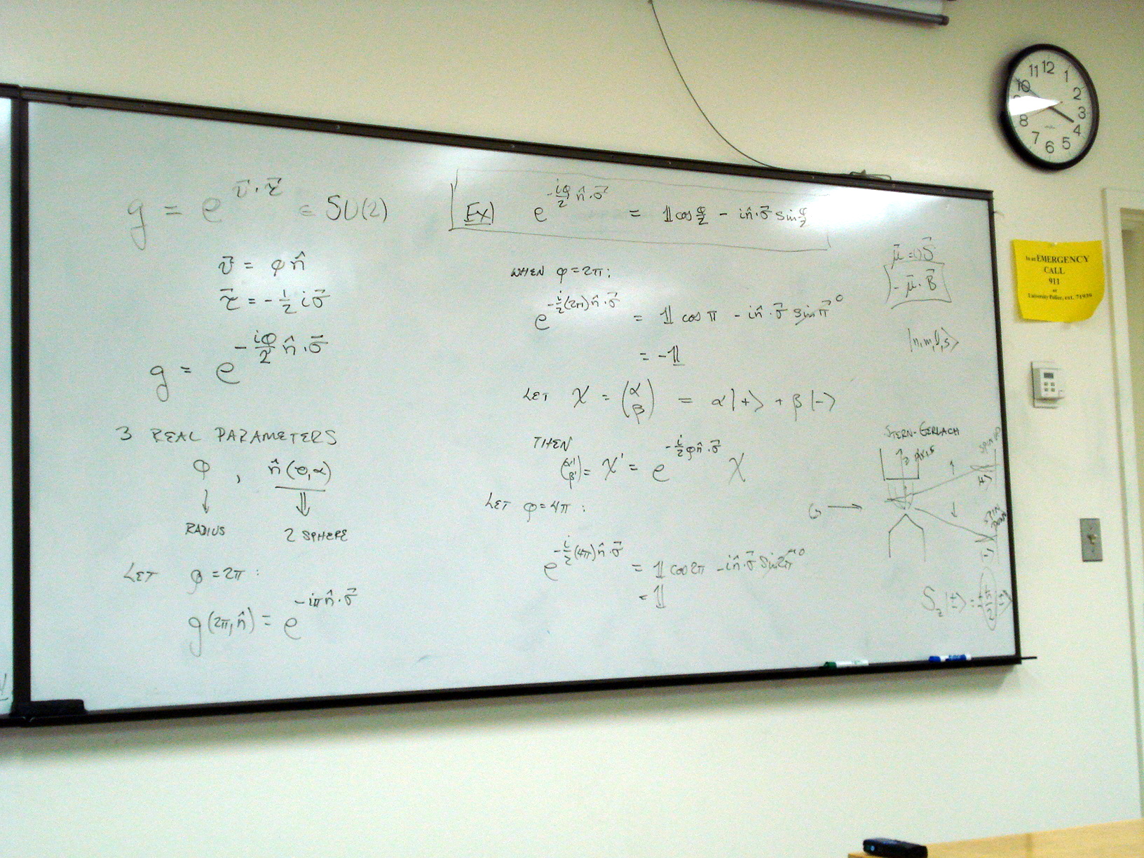
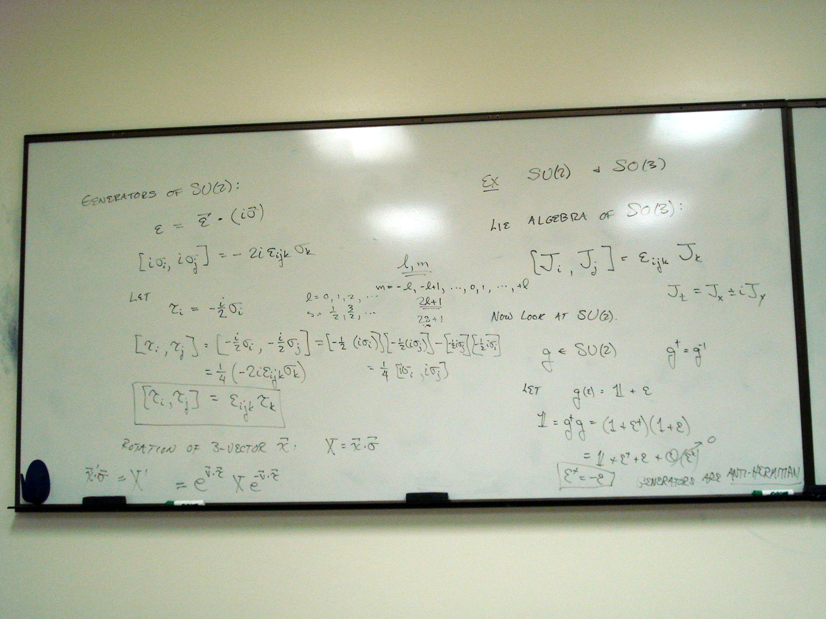
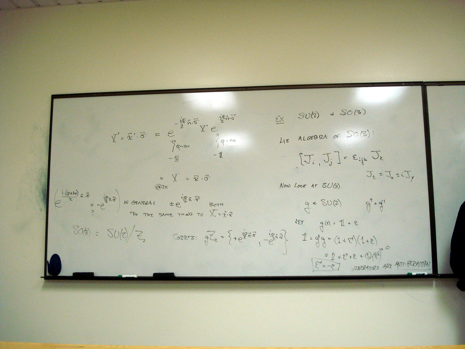
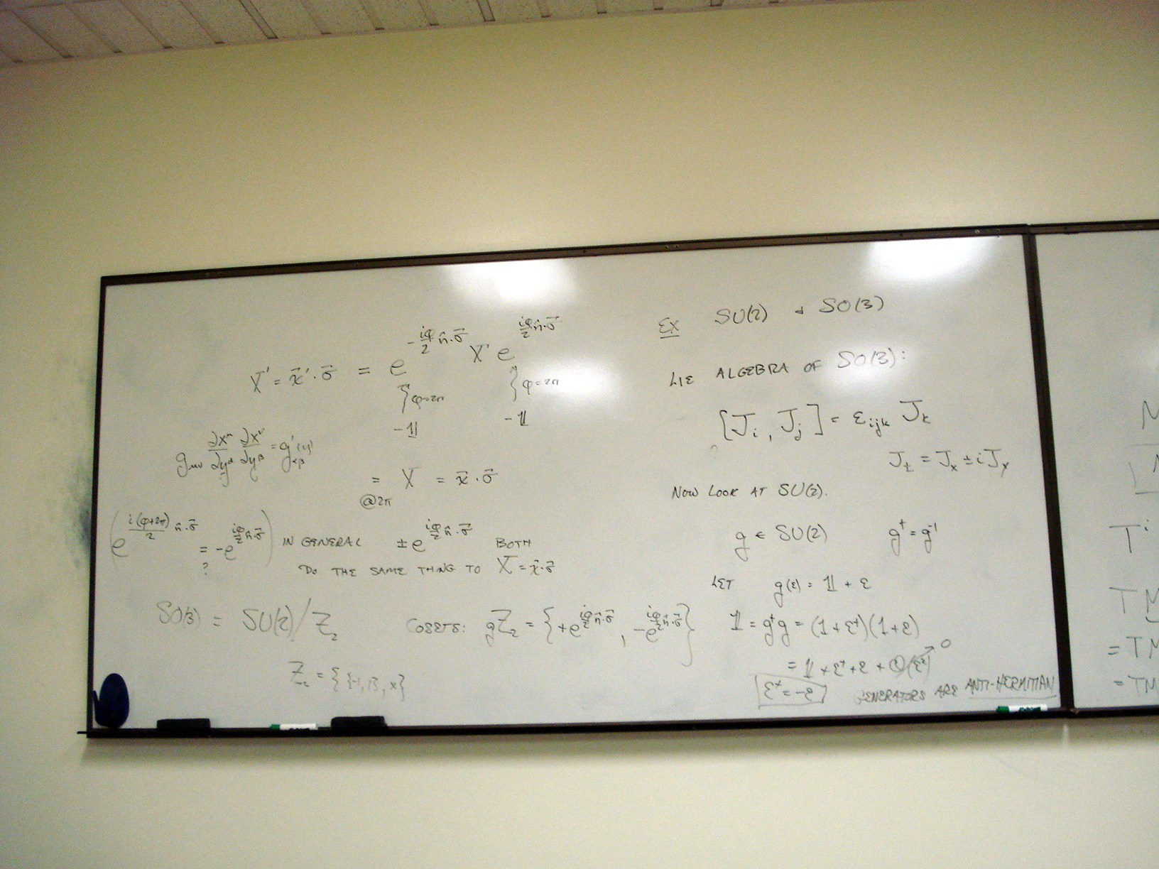
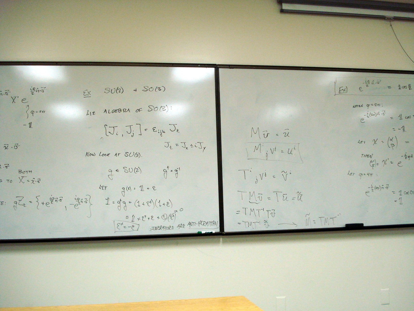
Notes: Irreducible
representations of the rotation group
Wednesday, February
11, 2009
Lecture:
Quotients by normal subgroups. Begin quotients by general subgroups.
Definition of a normal
subgroup. Theorem: the quotient of a group by a normal subgroup is a group.
Proof.
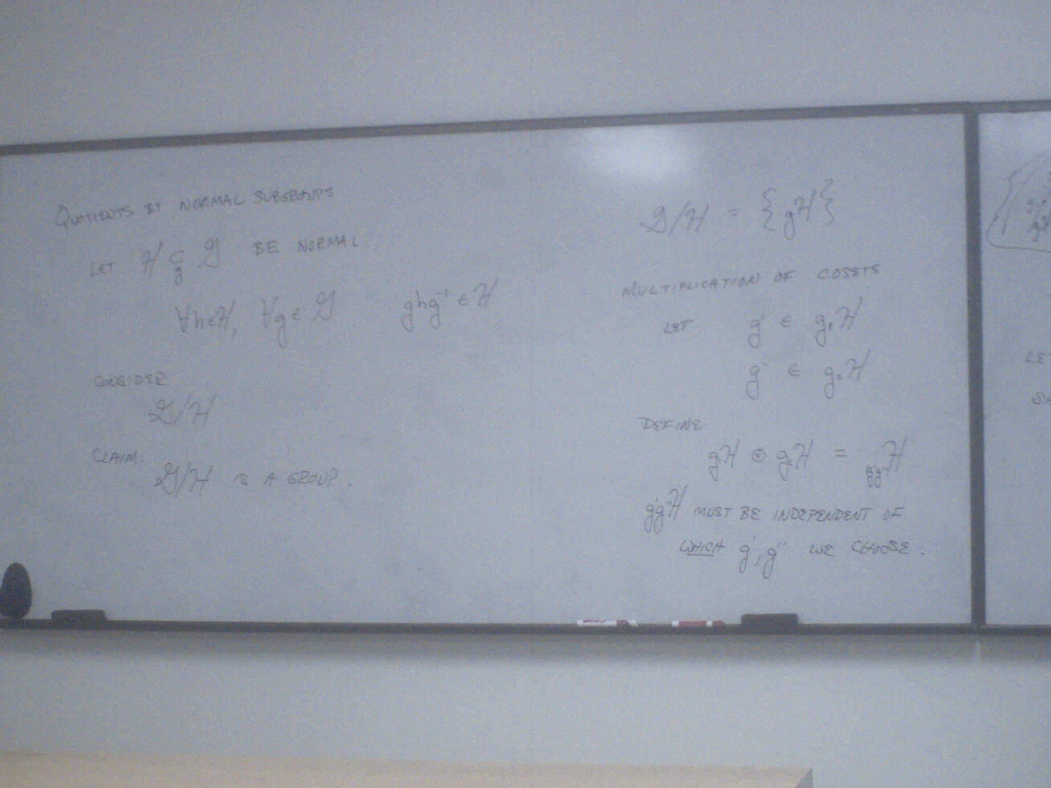
Proof (duplicate photos)
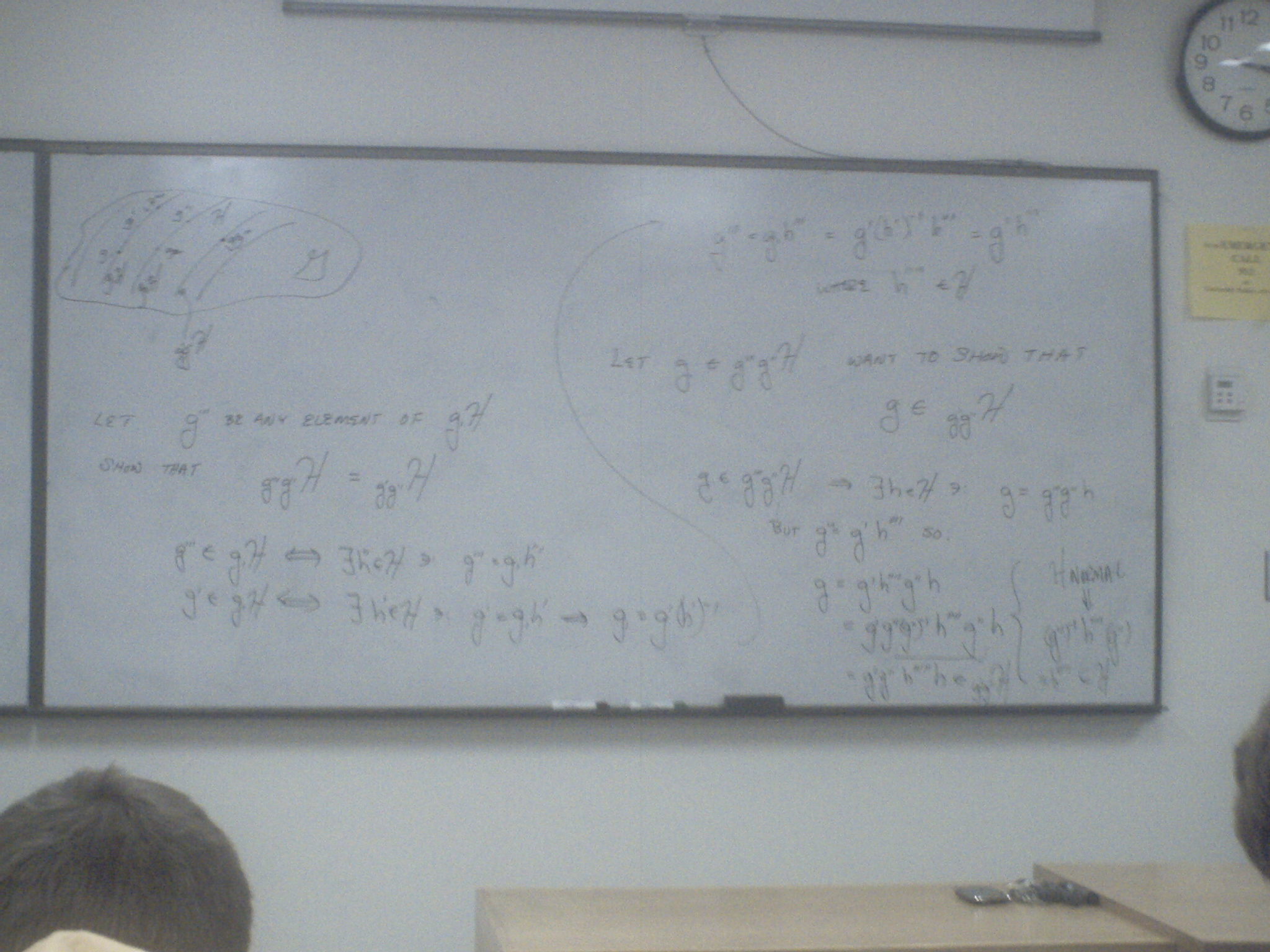
Example: GL(n) has a
normal subgroup, H, consisting of multiples of the identity. The quotient
GL(n)/H is SL(n):
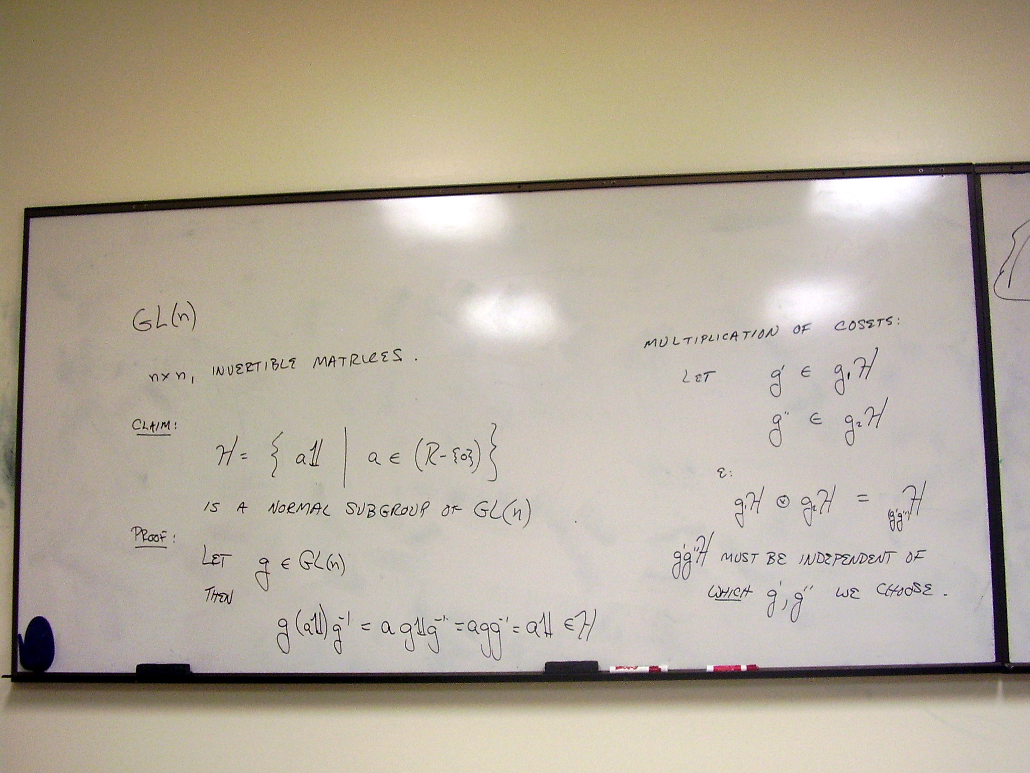
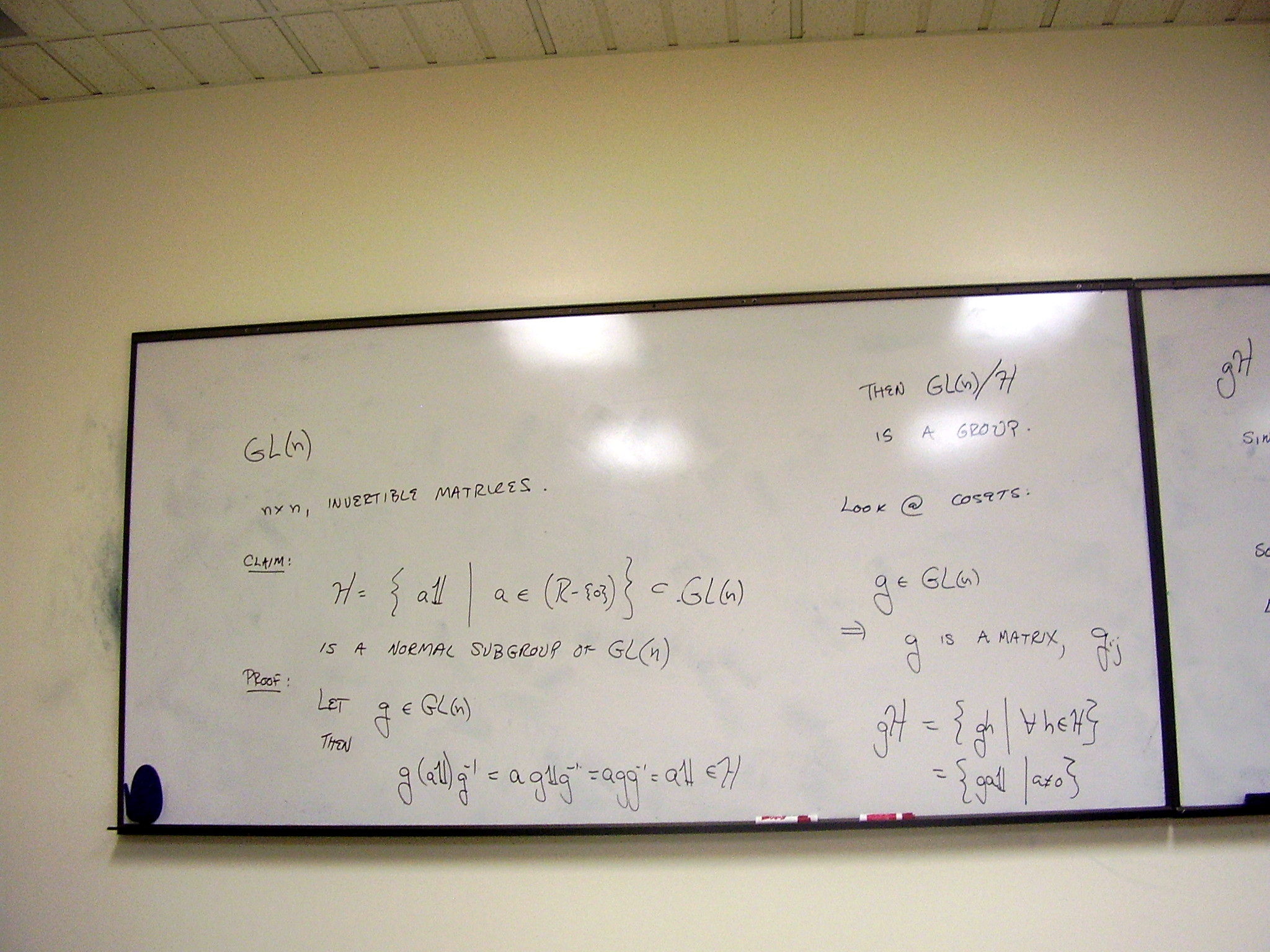
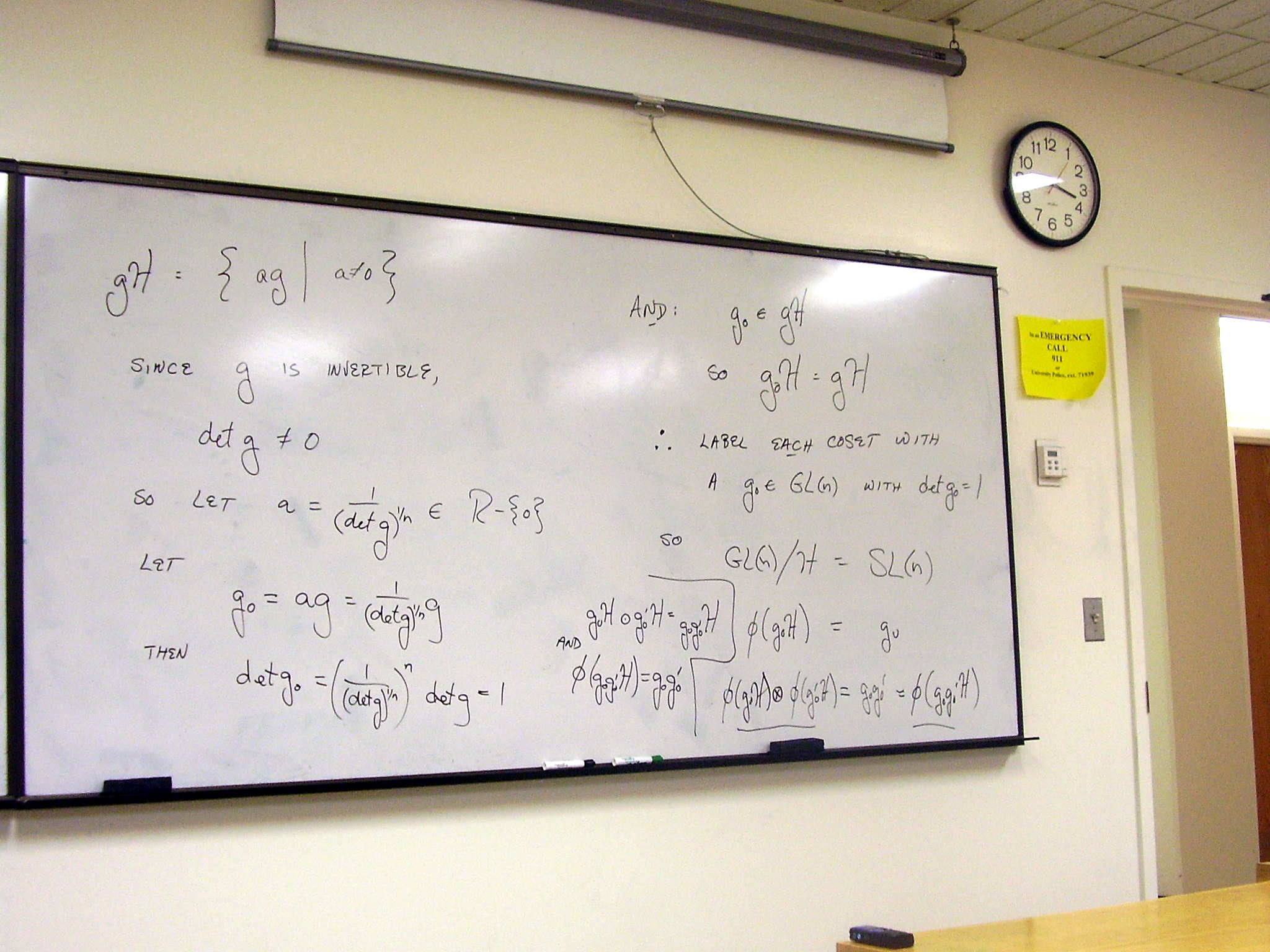
Cosets are homomorphic:
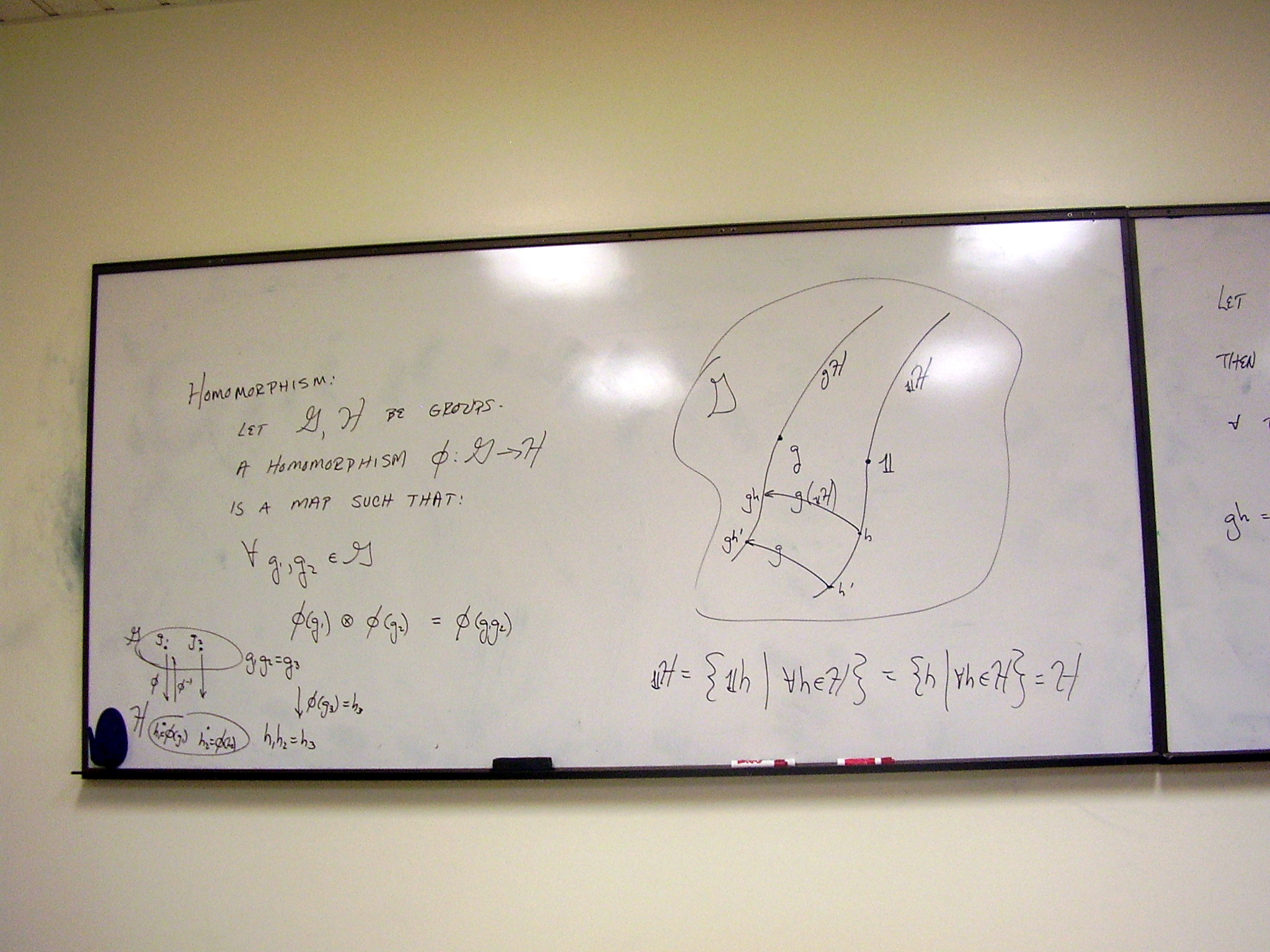
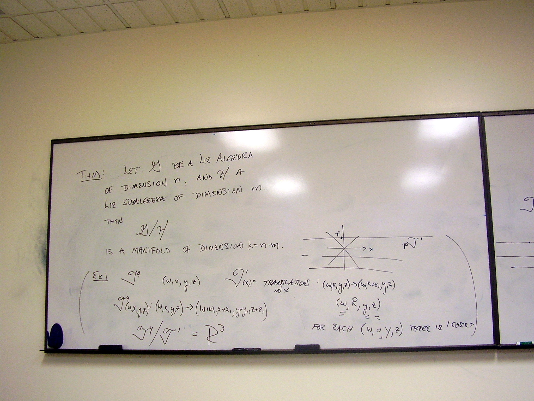
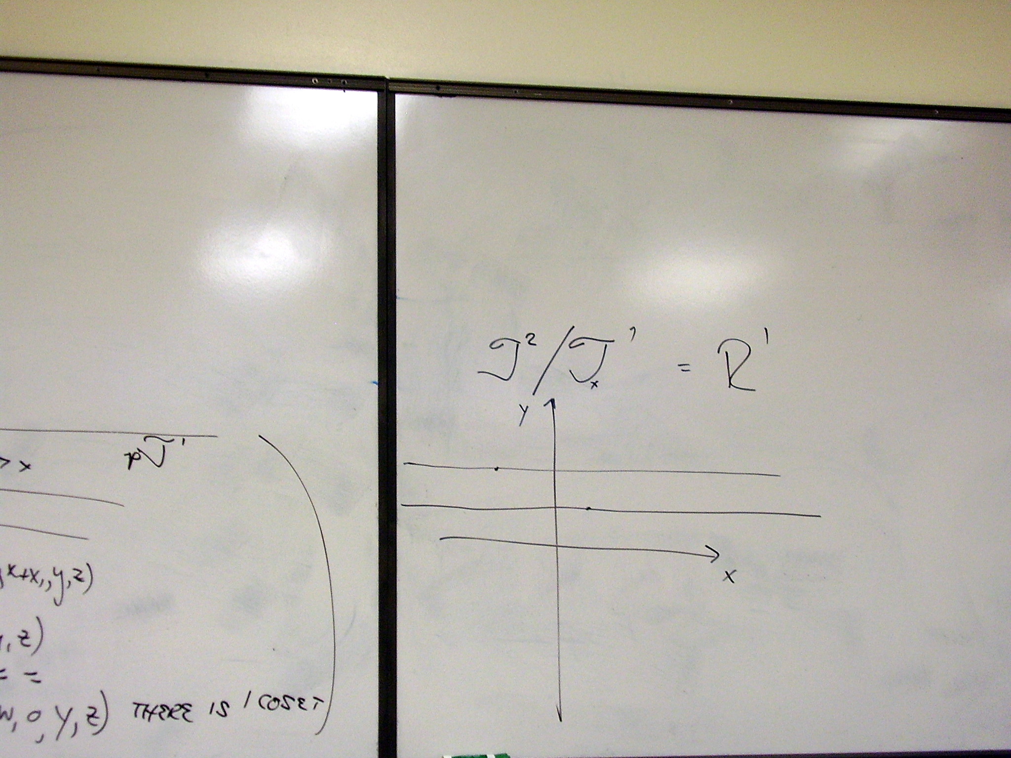
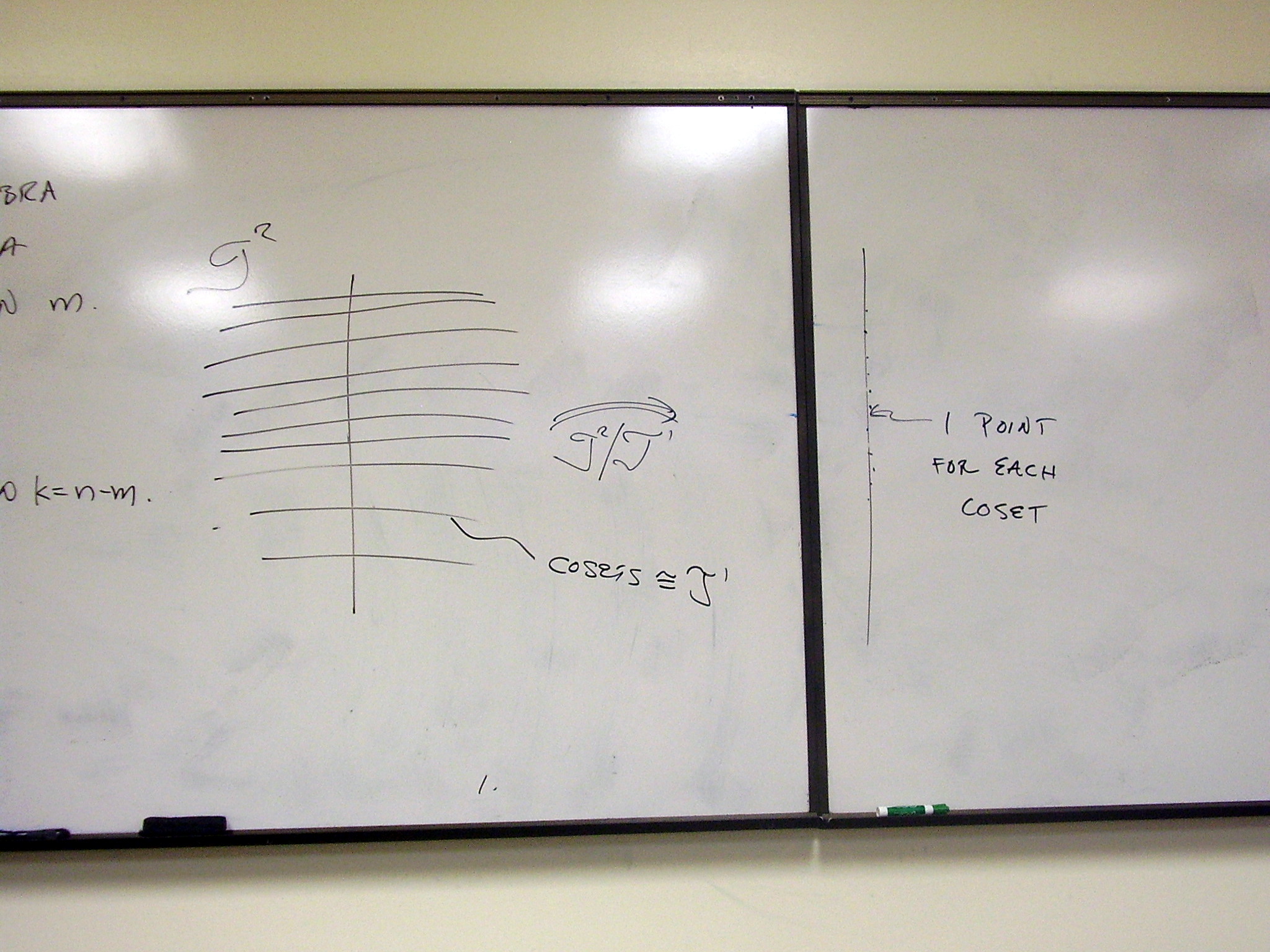
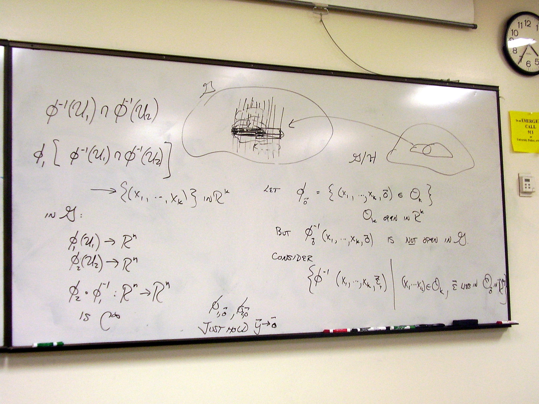
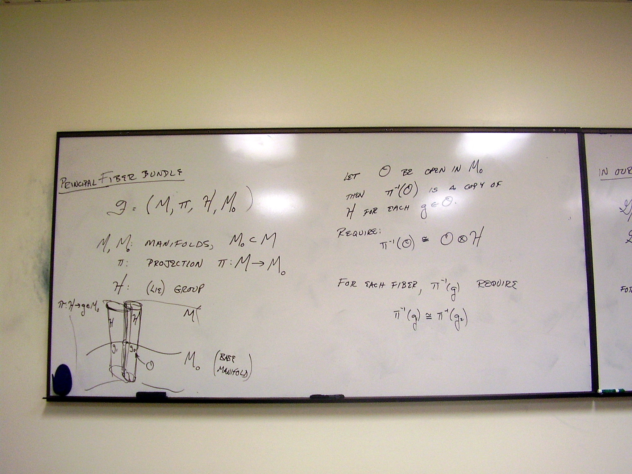
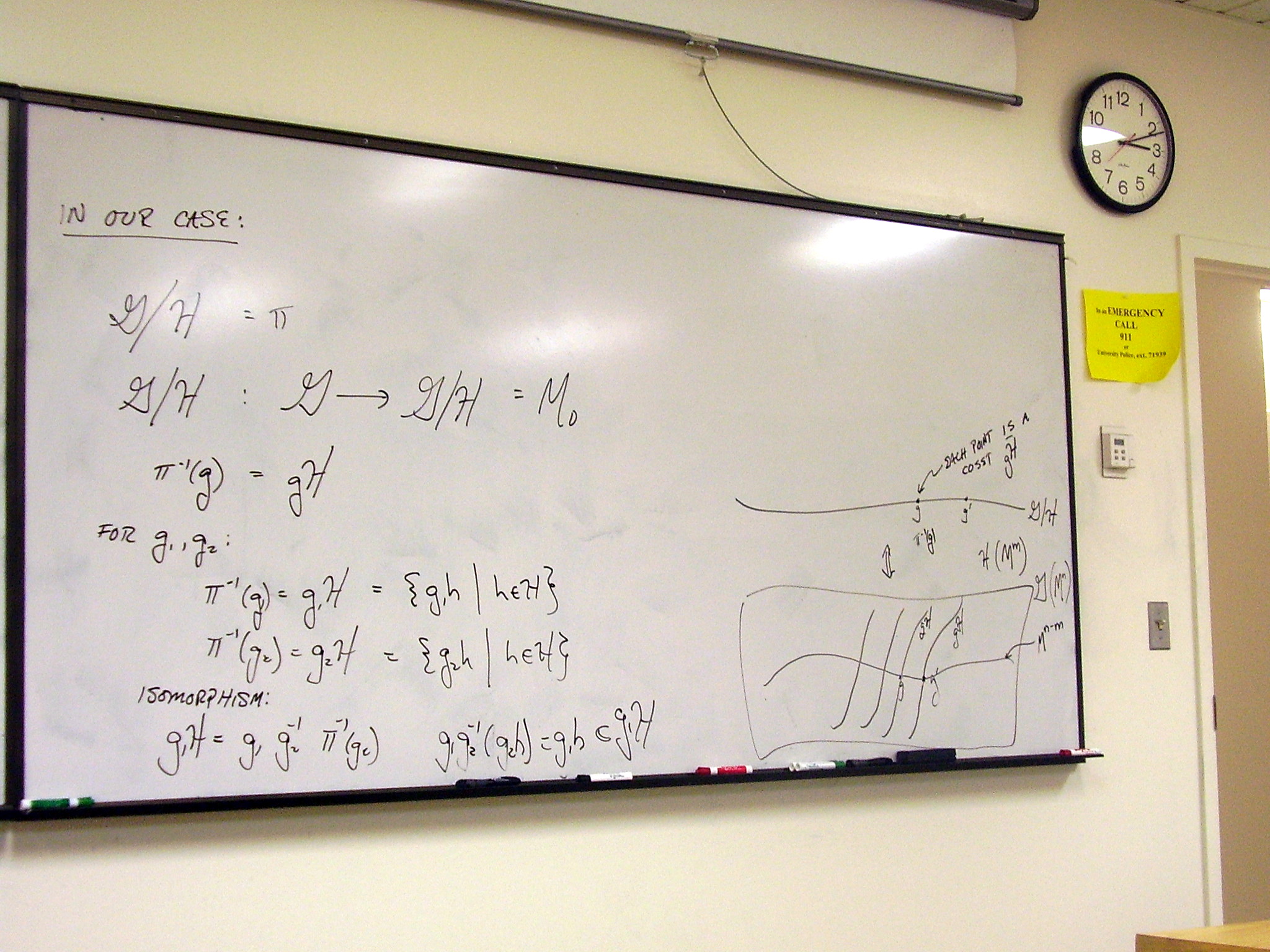
Central theorem: The
quotient of a Lie group by a Lie subgroup is a manifold. Discussion:
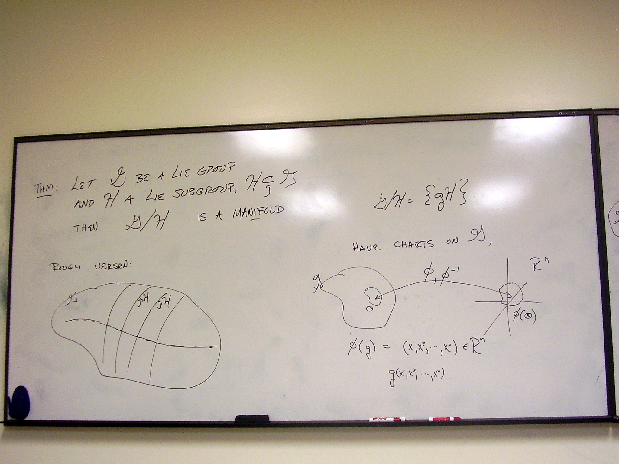
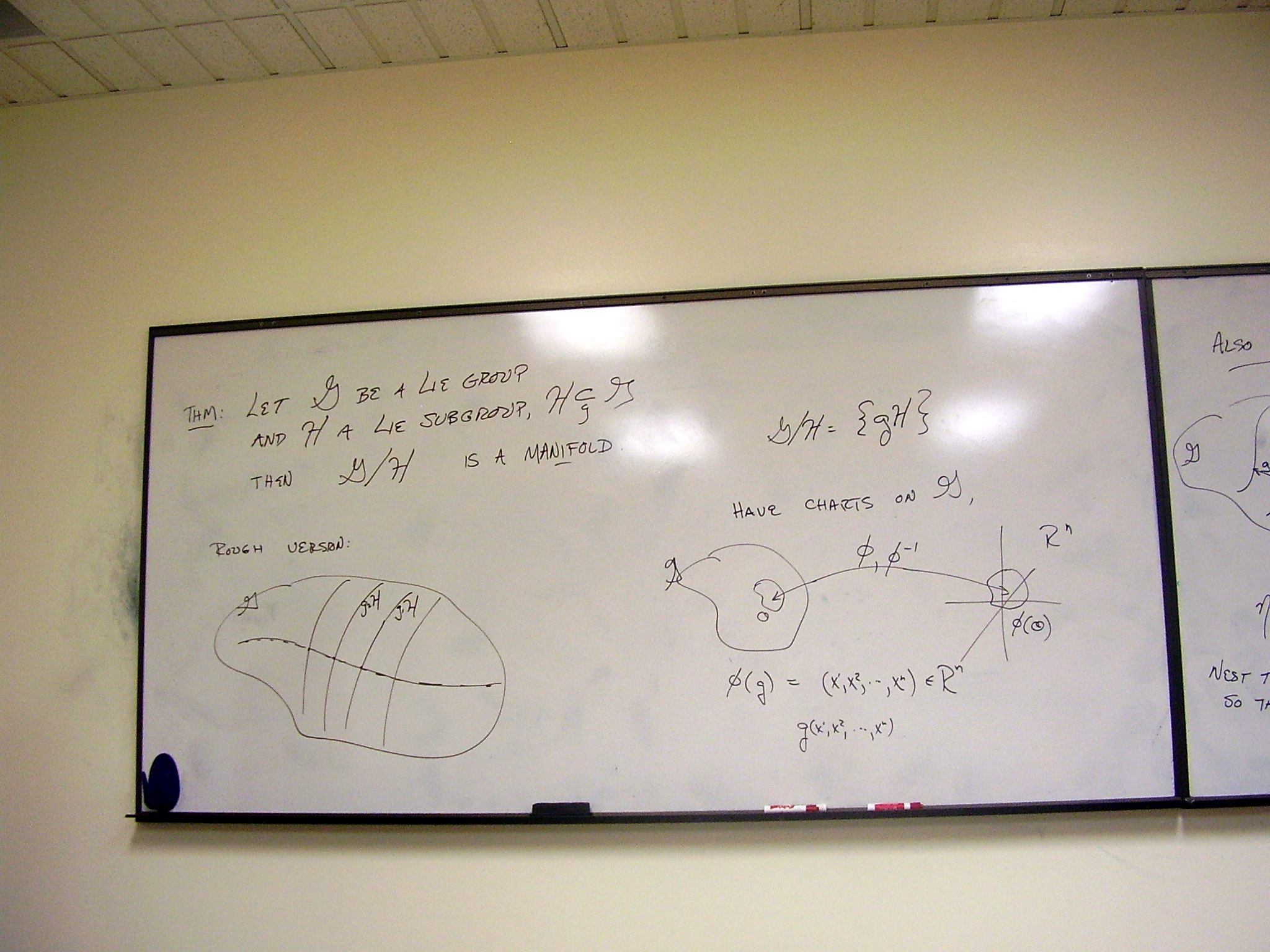
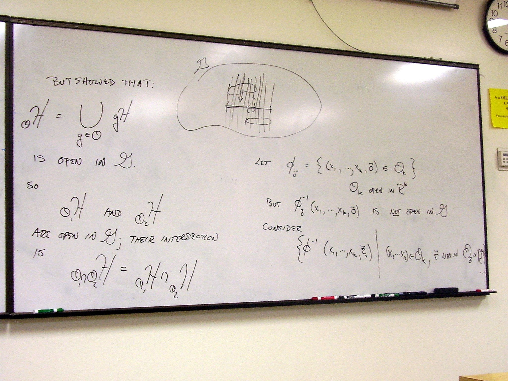
The “rod” over an open set
(technically, the inverse projection) is an open set:
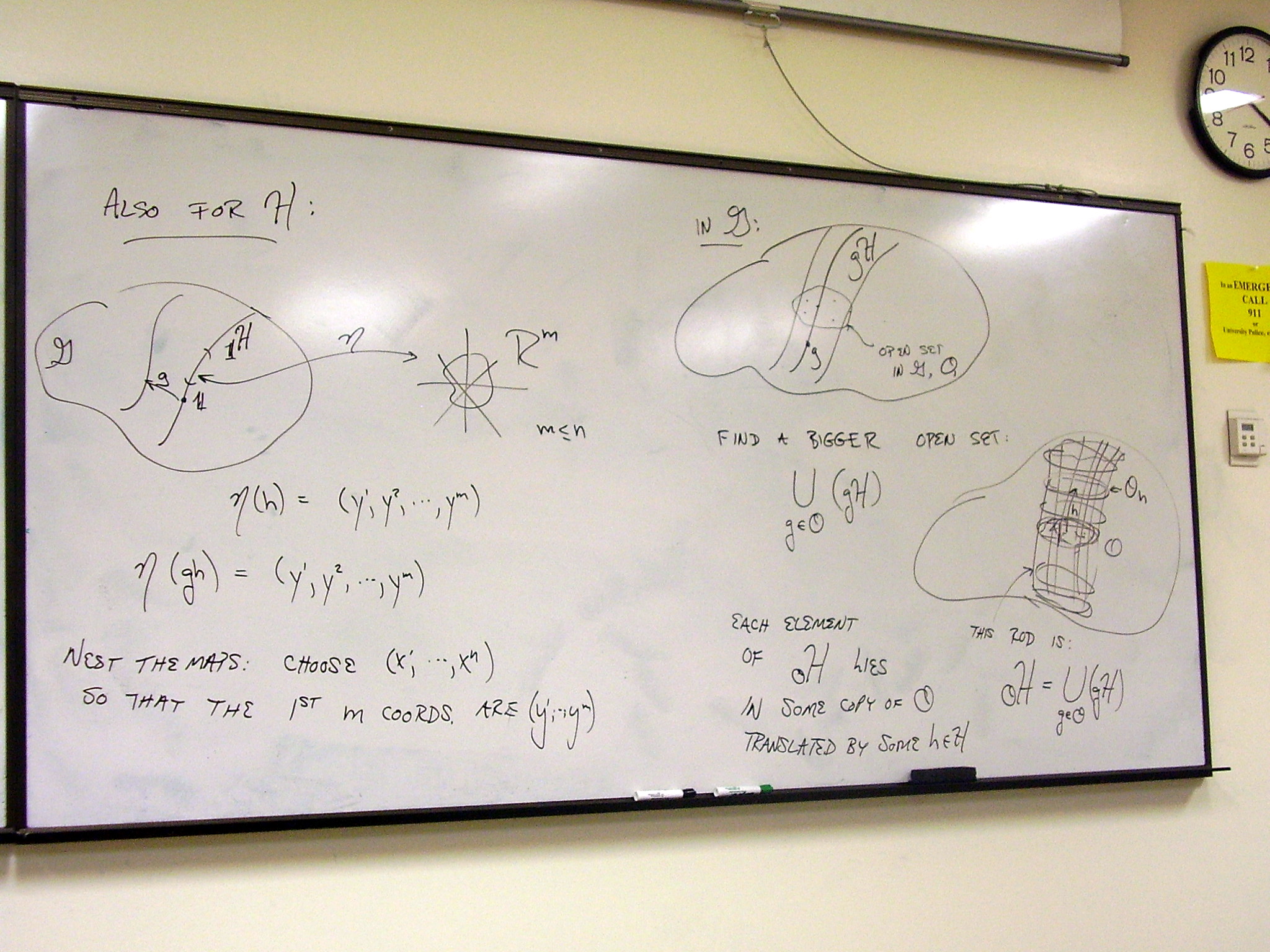
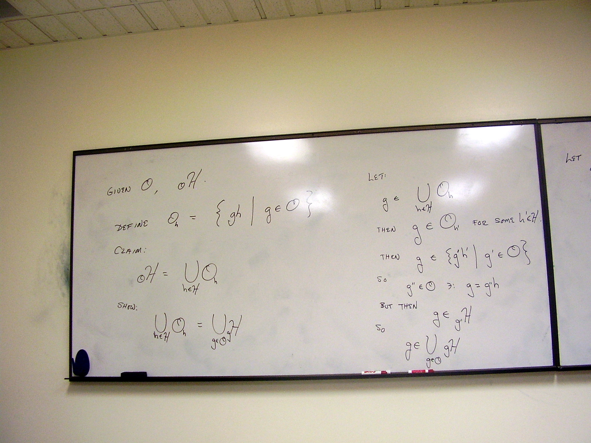
Friday, February 13,
2009
Lecture:
The quotient of a Lie group by a Lie subgroup is a manifold
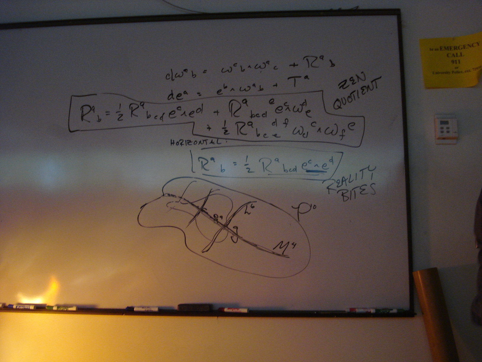
One advantage of
differential forms: the Riemann curvature tensor in coordinates, vs. the
Riemann curvature 2-form
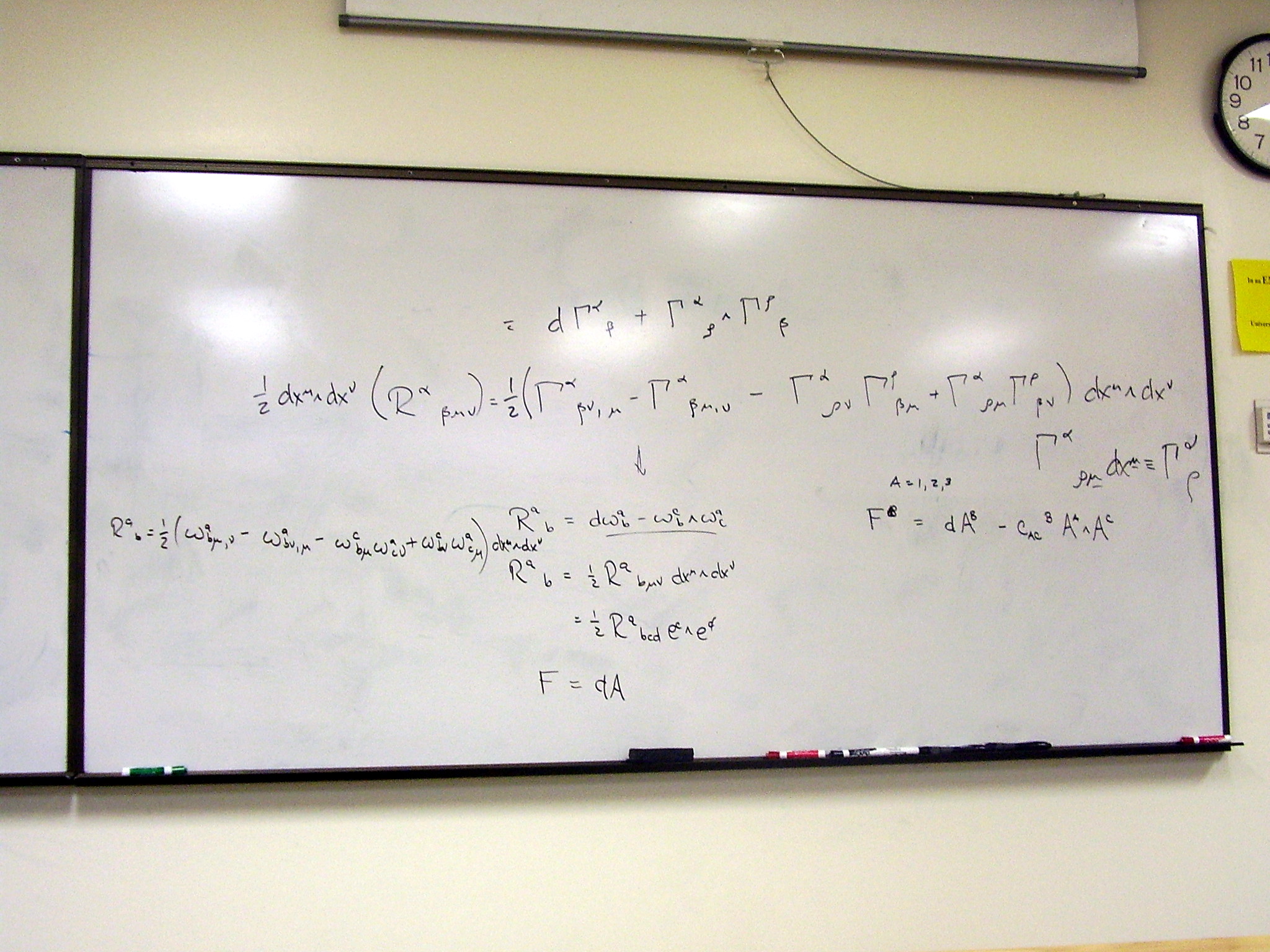
Structure constants for the
Lorentz group:
Theorem: the quotient of a
Lie group by a Lie subgroup is a manifold. A simple example
Exercise: check that the
theorem holds when the subgroup is normal.
Proof of the theorem.
(Choose coordinates adapted to the quotient)
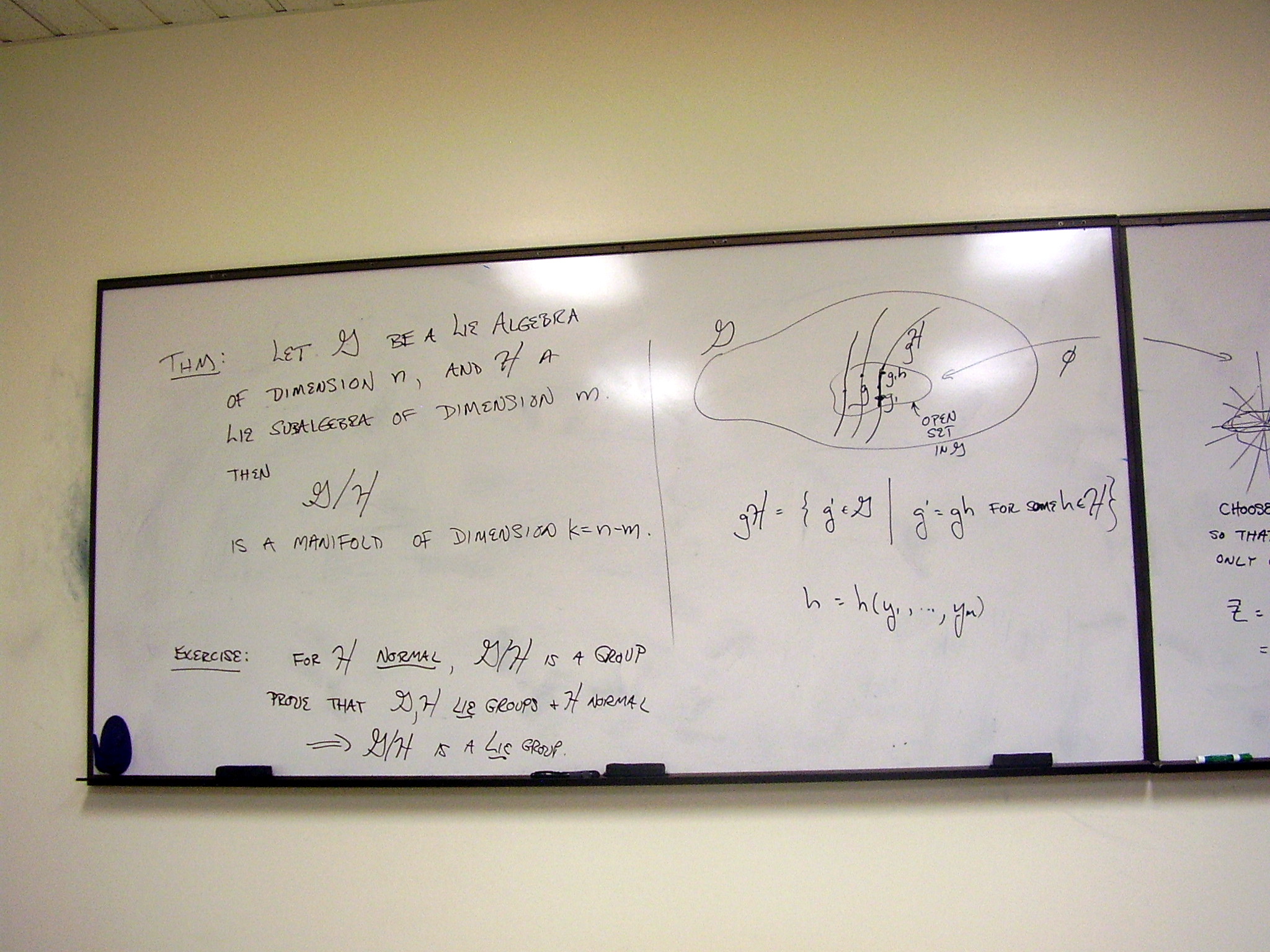
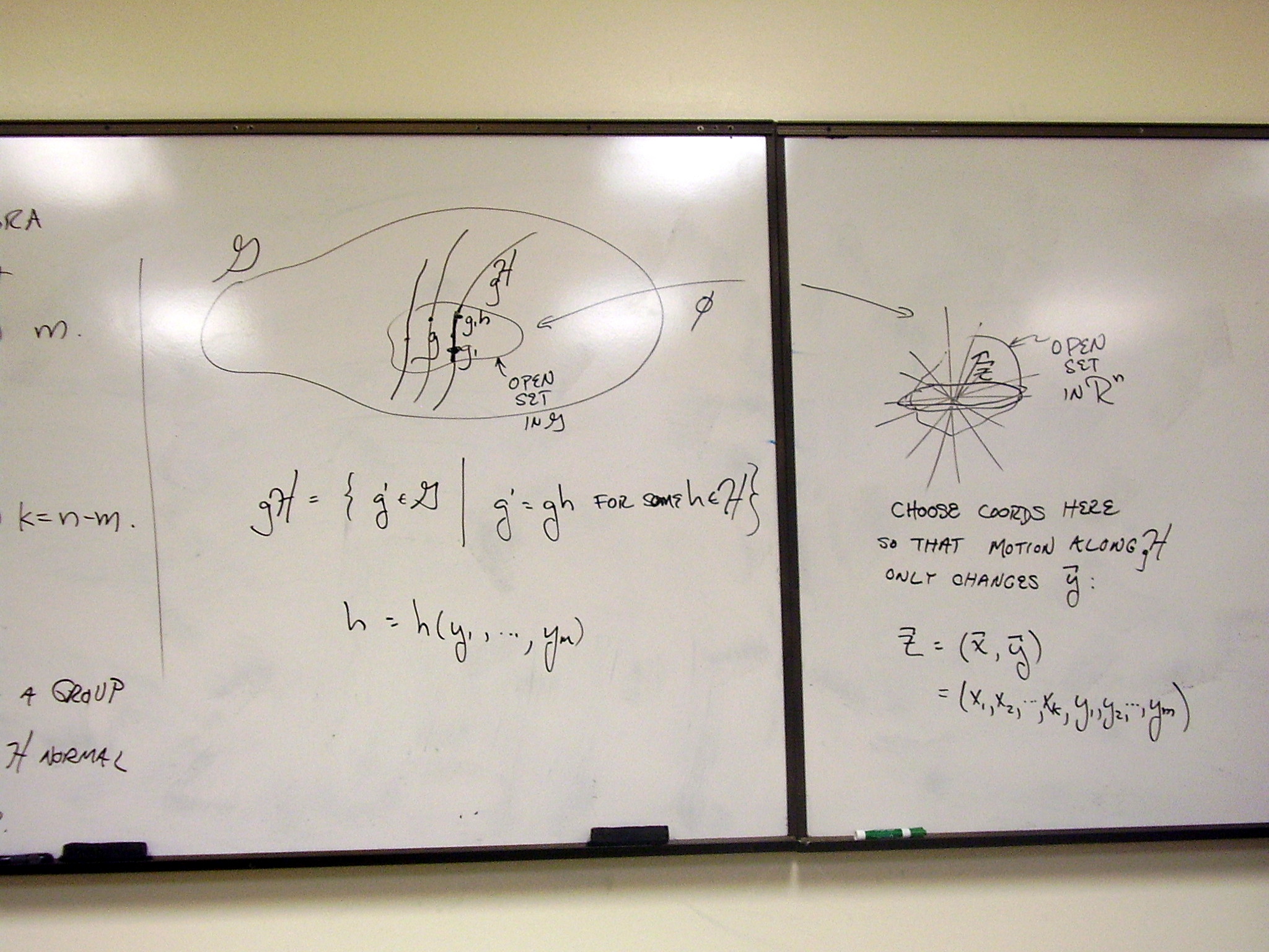
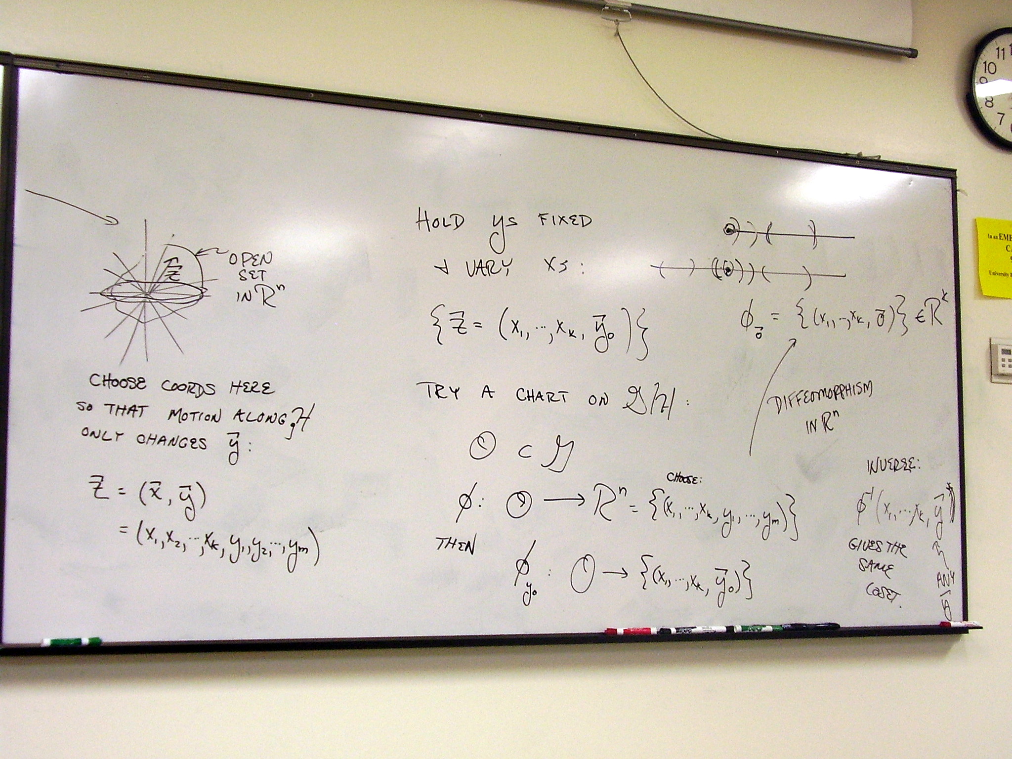
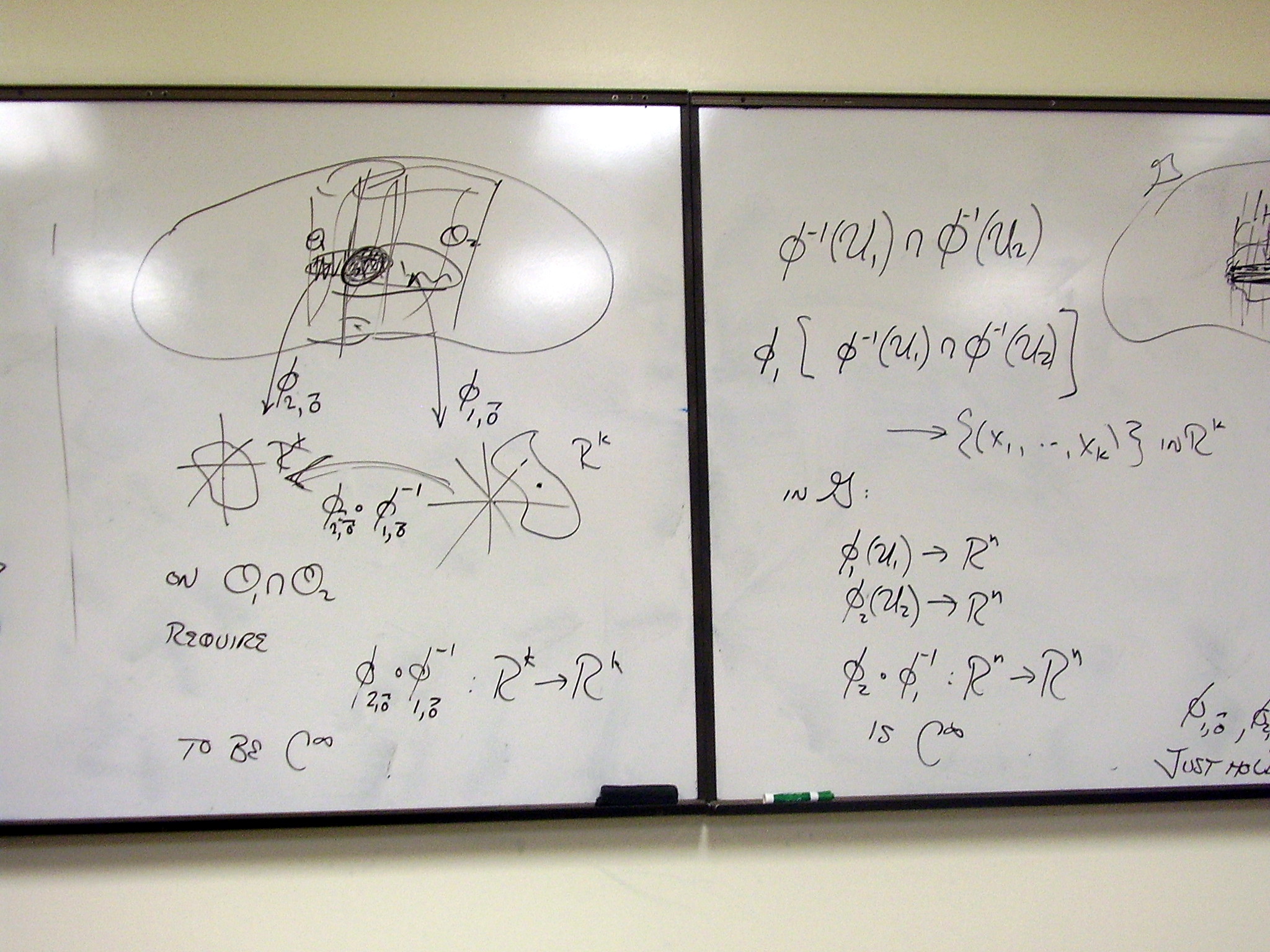
C. Gauge
theory
Tuesday, February 17,
2009
Fiber bundles. The quotient
of Lie groups is an easy case.
Overview: From Lie algebra
to Maurer-Cartan equations to fiber bundle to gauge theory.
Gauge theory from the
invariance of an action.
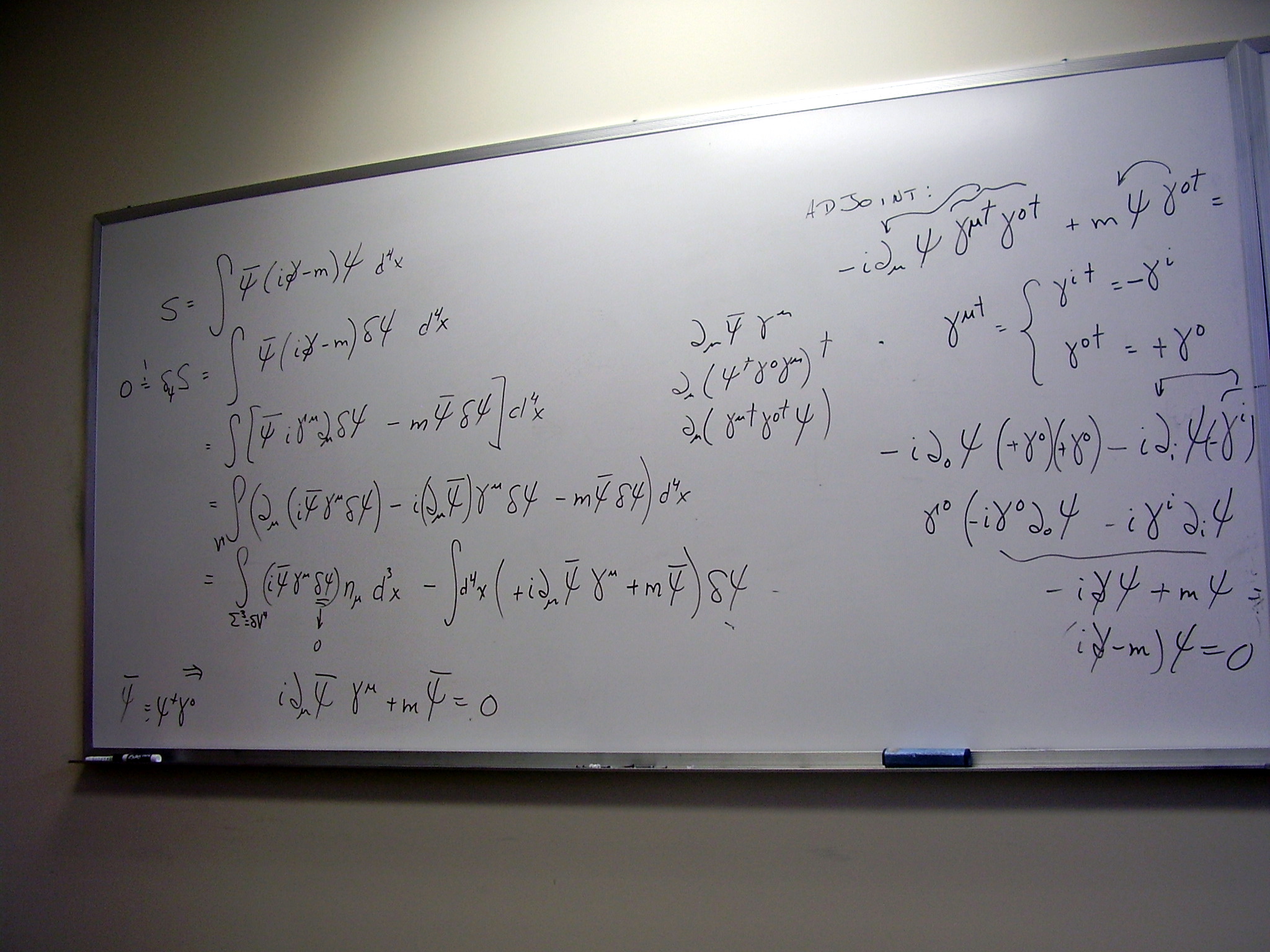
The Dirac equation as the
square root of the Klein-Gordon equation:
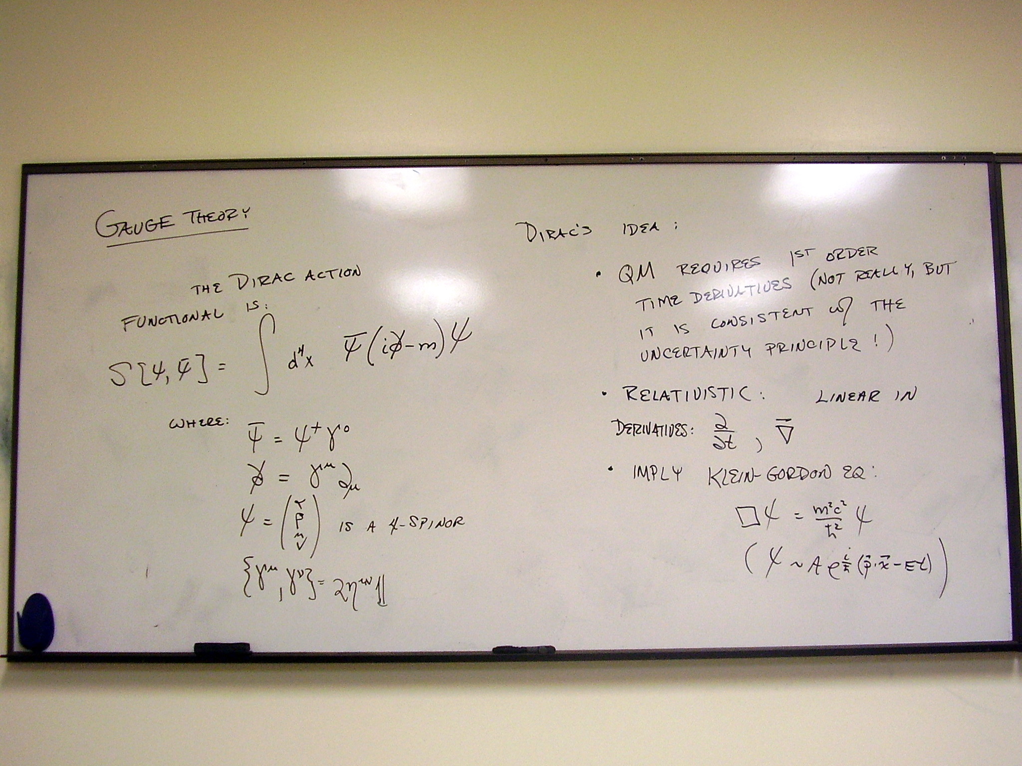
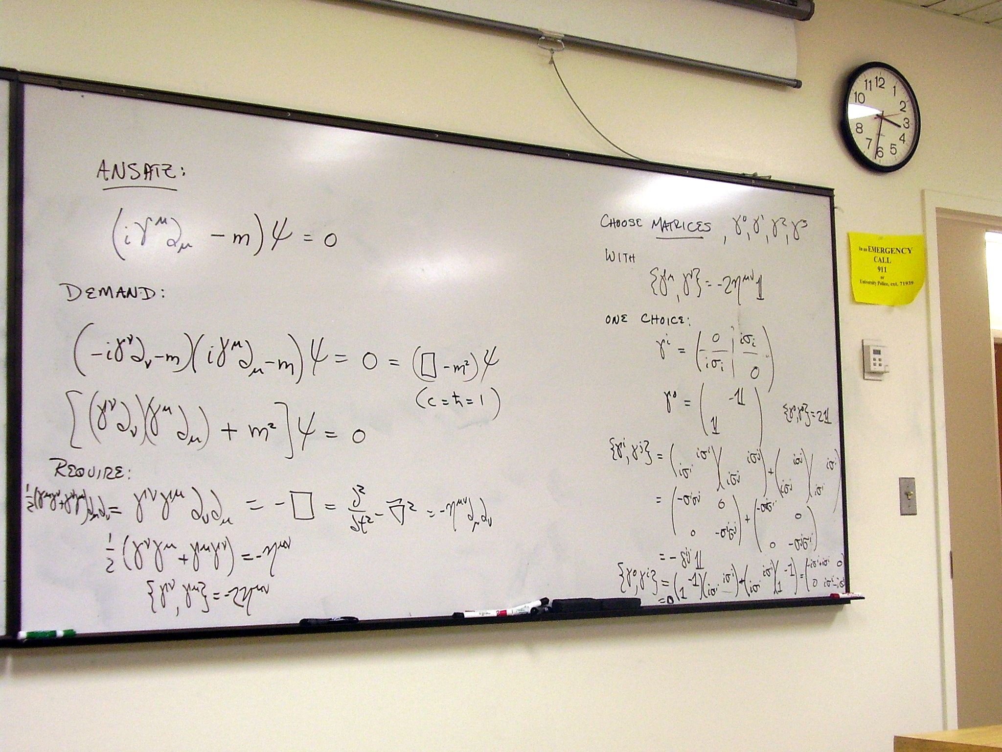
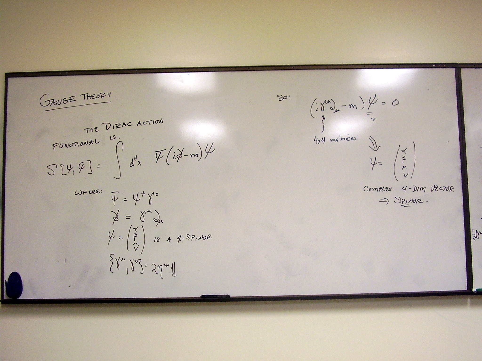
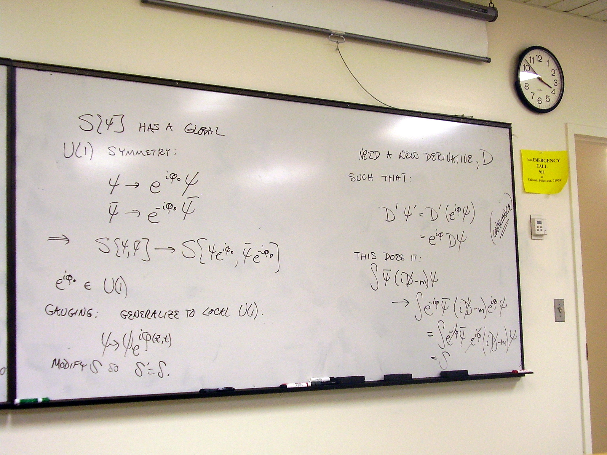
The Dirac equation (and
its conjugate) from an action:
Global U(1) invariance of
the Dirac action. Generalizing to local U(1) symmetry. The invariant field
strength and the modified action. The resulting fiber bundle.
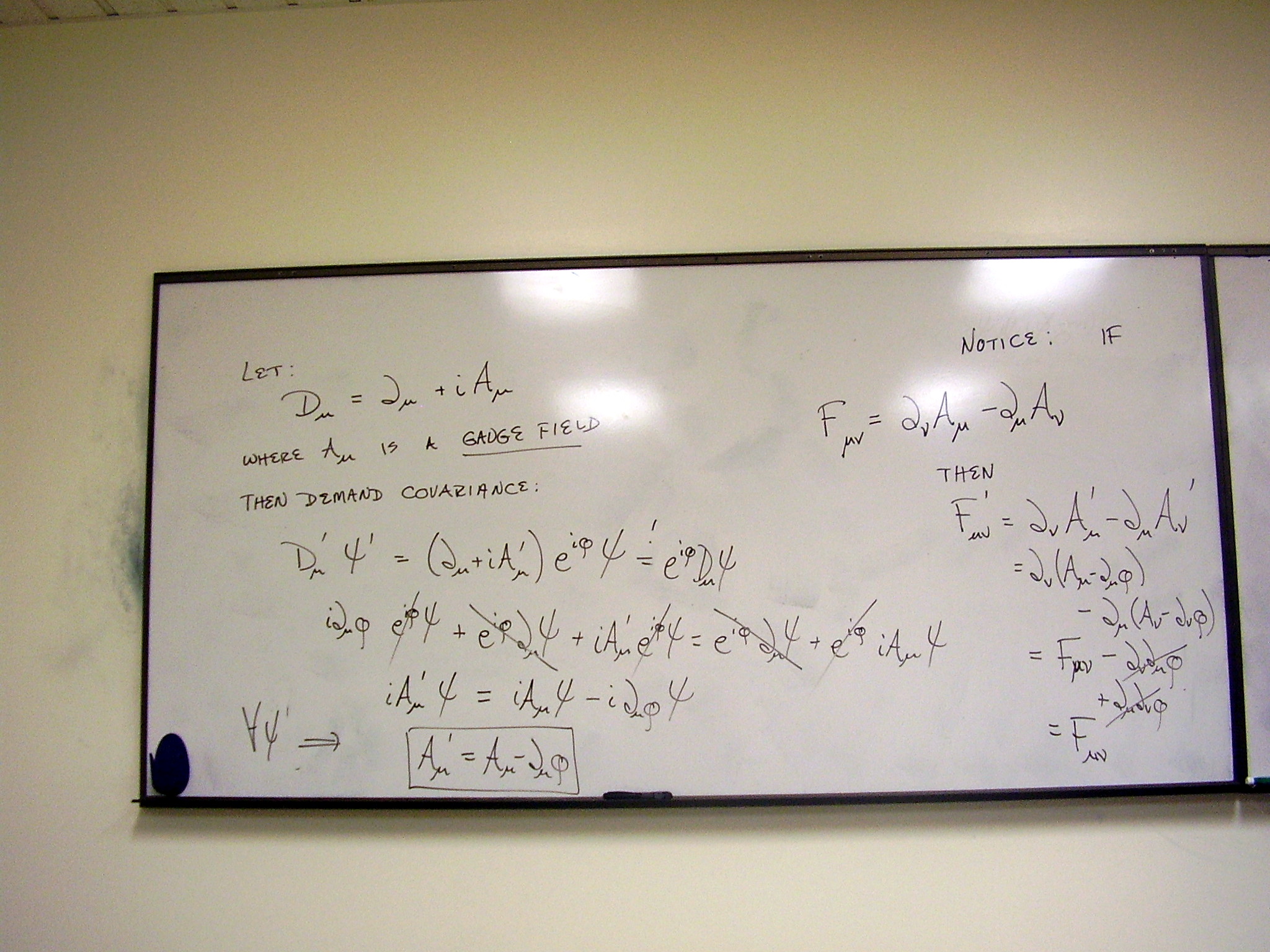
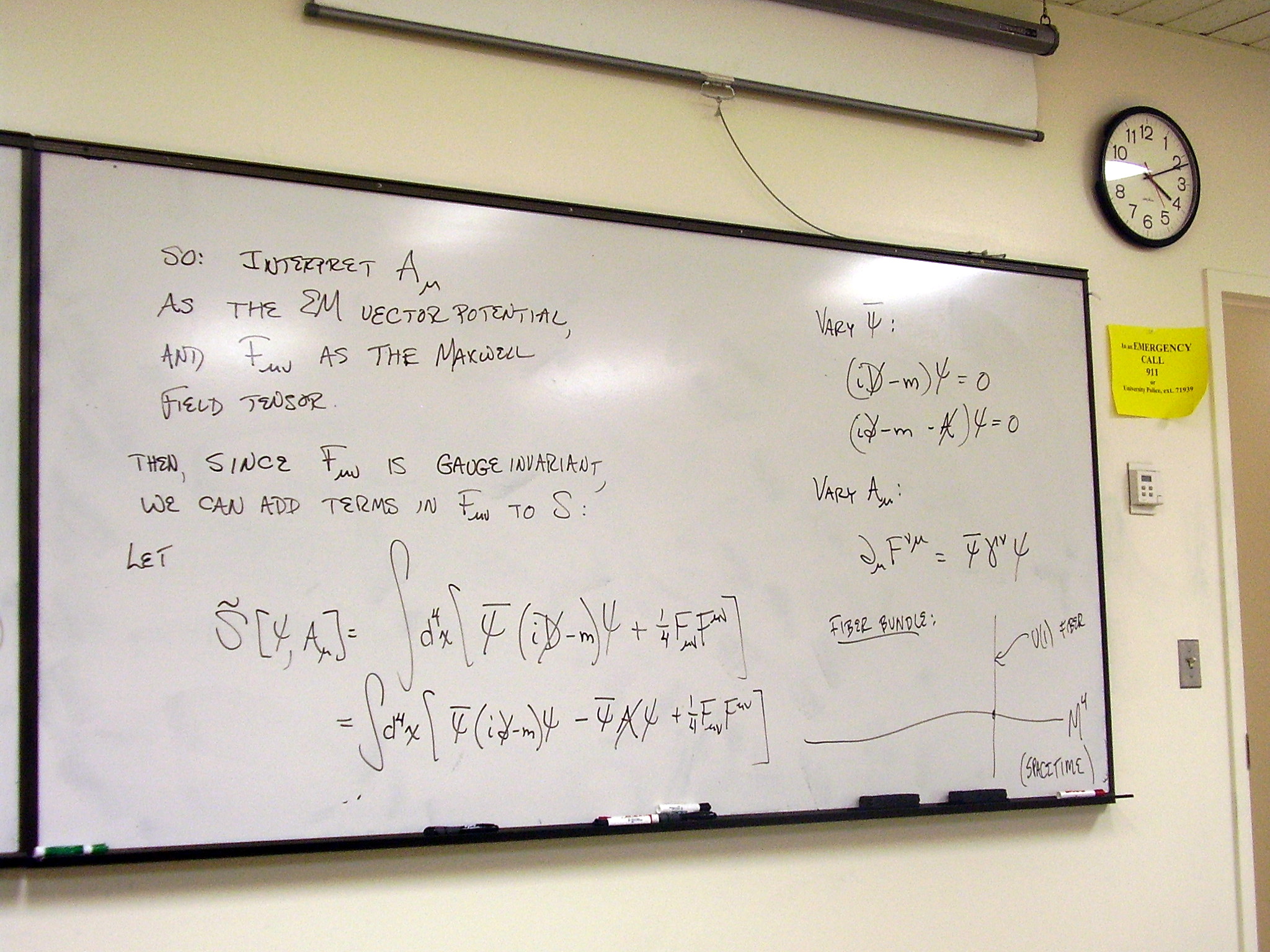
Wednesday, February
18, 2009
Lecture:
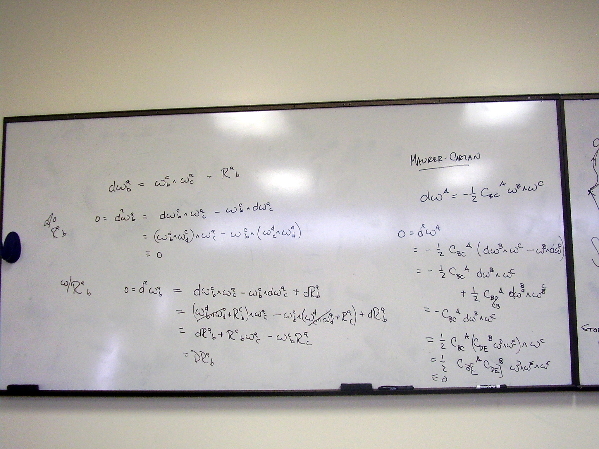
The Maurer-Cartan structure equations
Variation of the Dirac
action (detail)
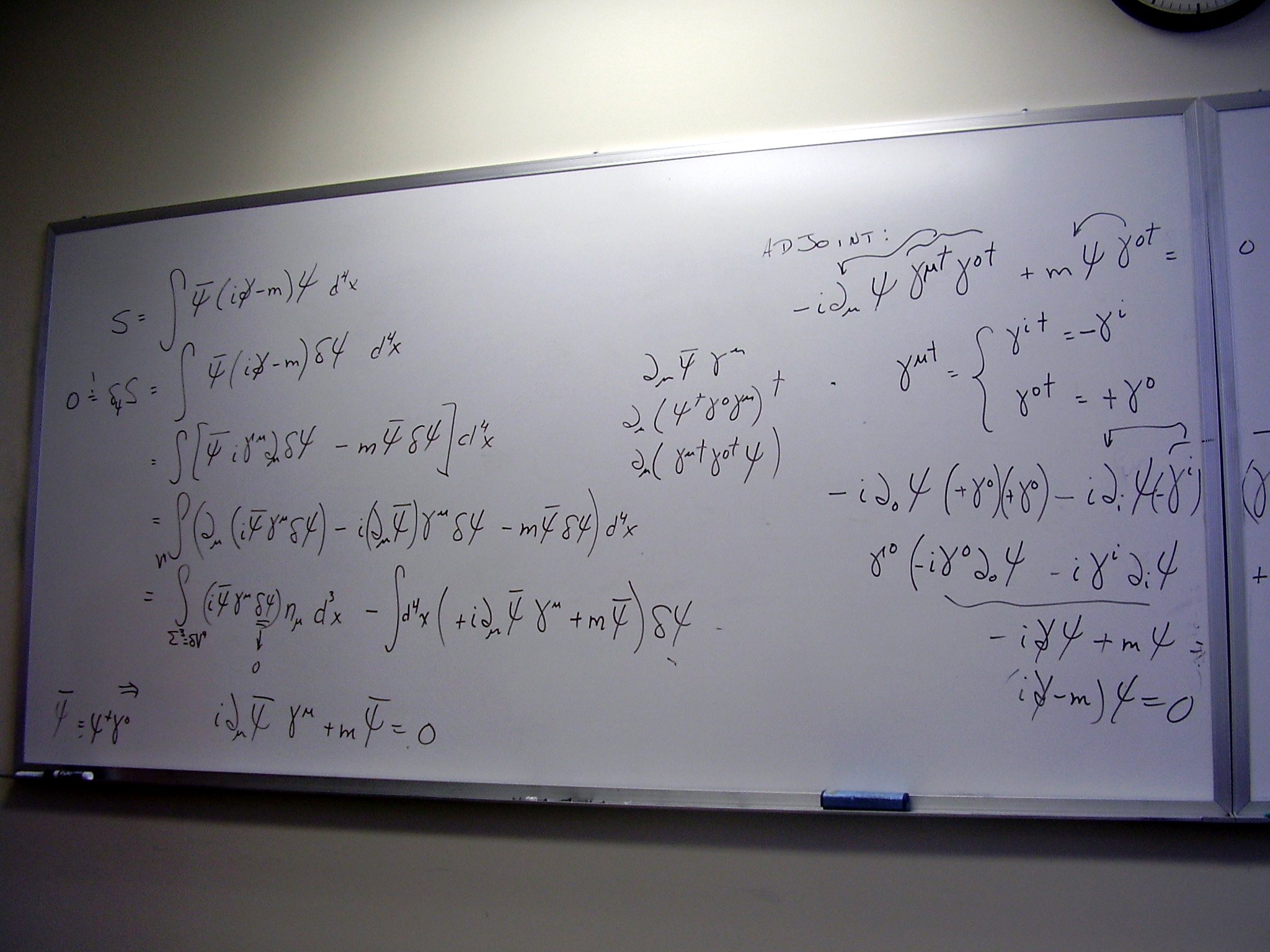
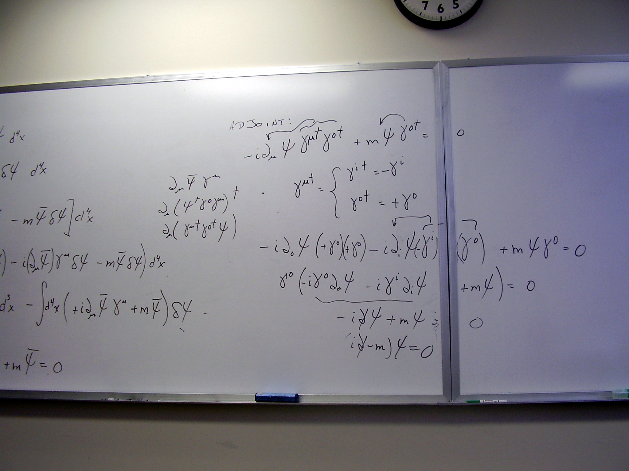
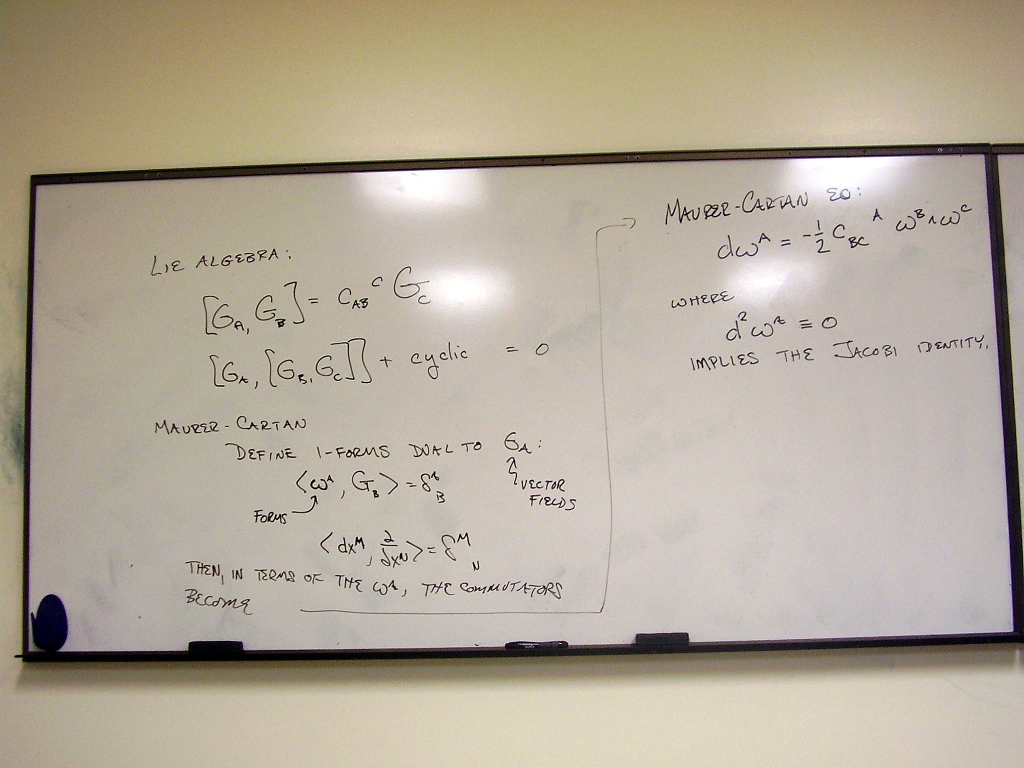
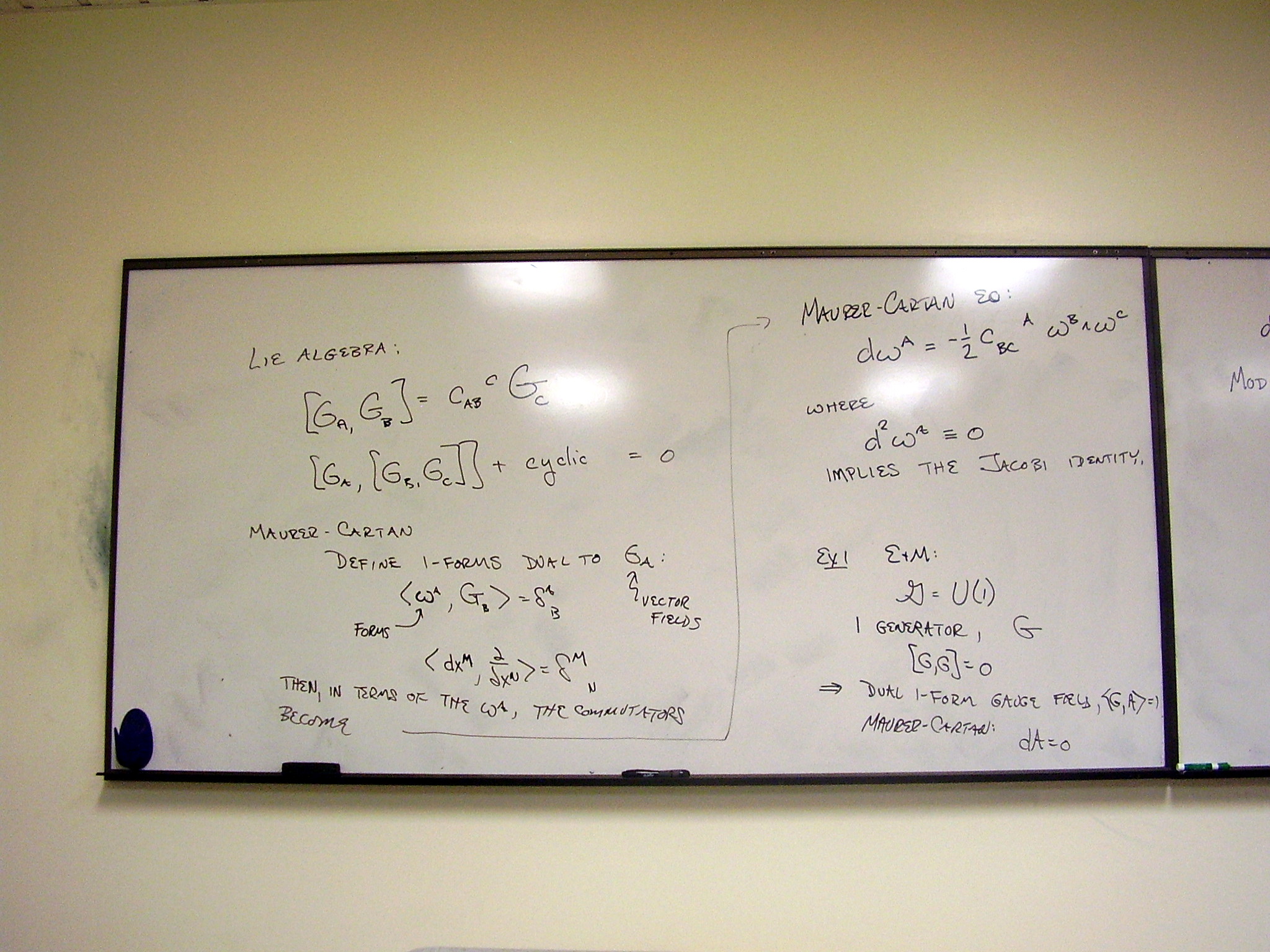
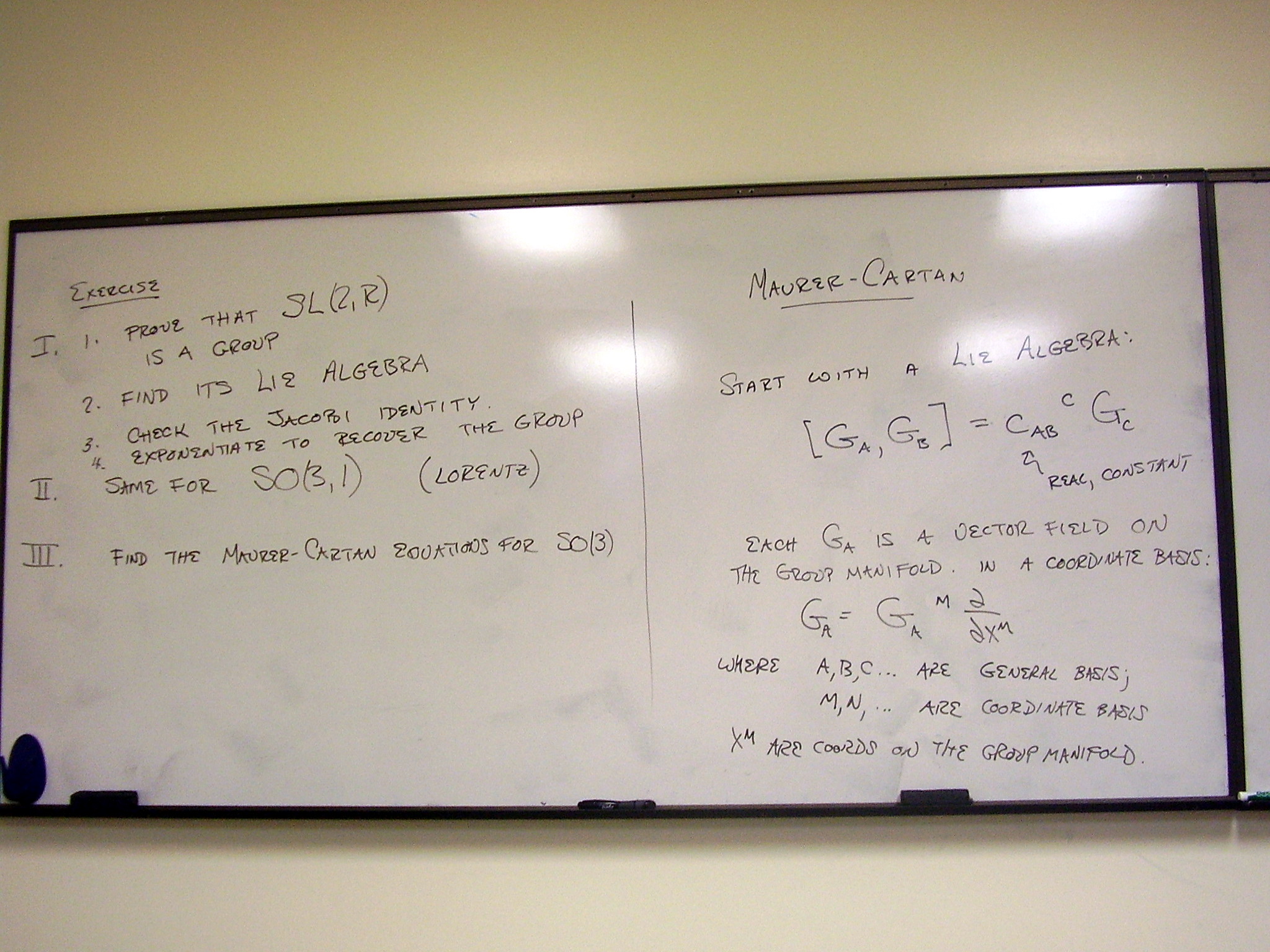
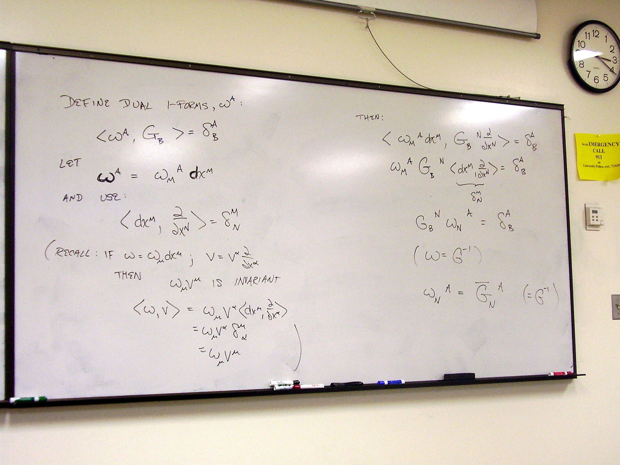
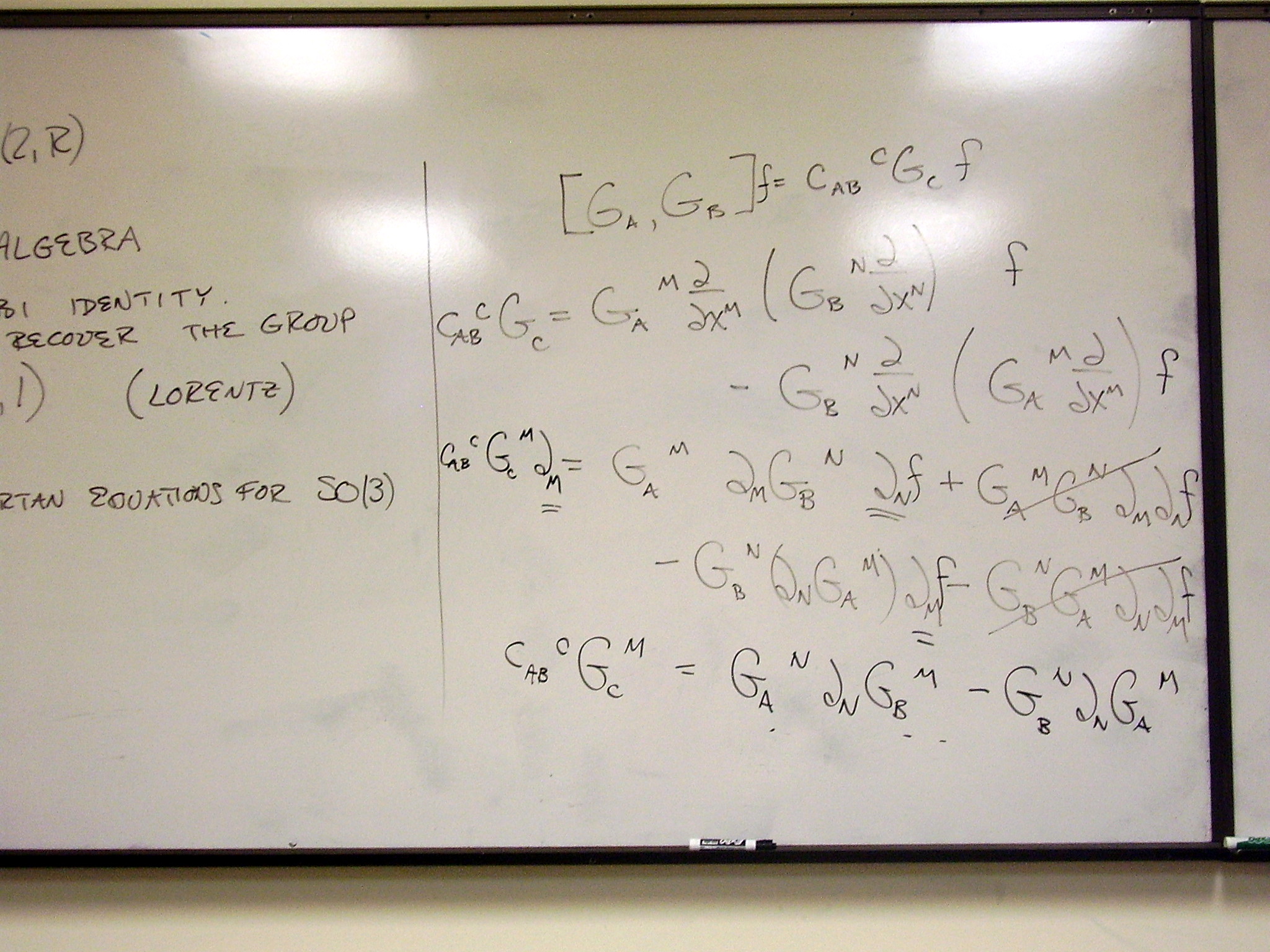
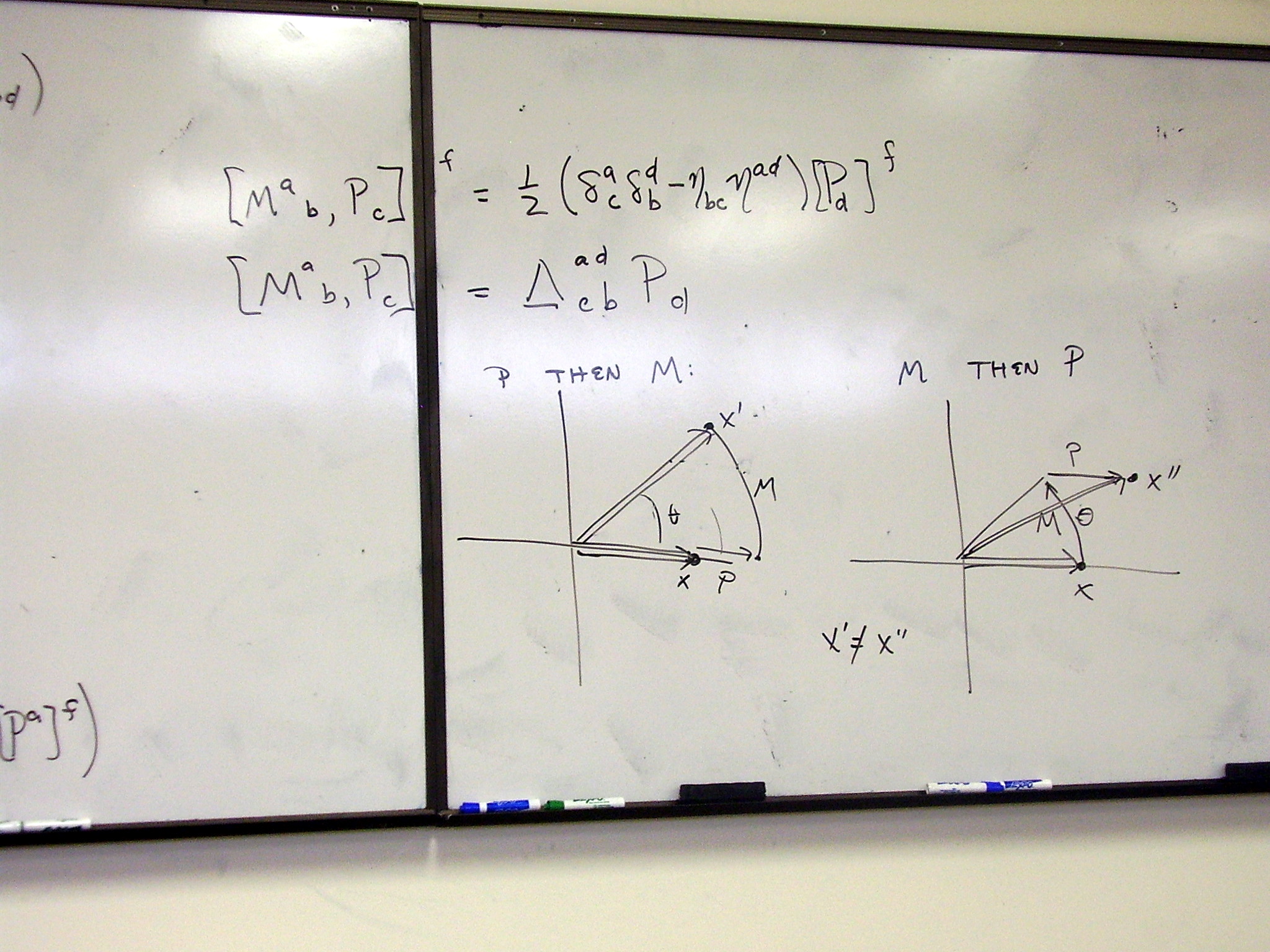
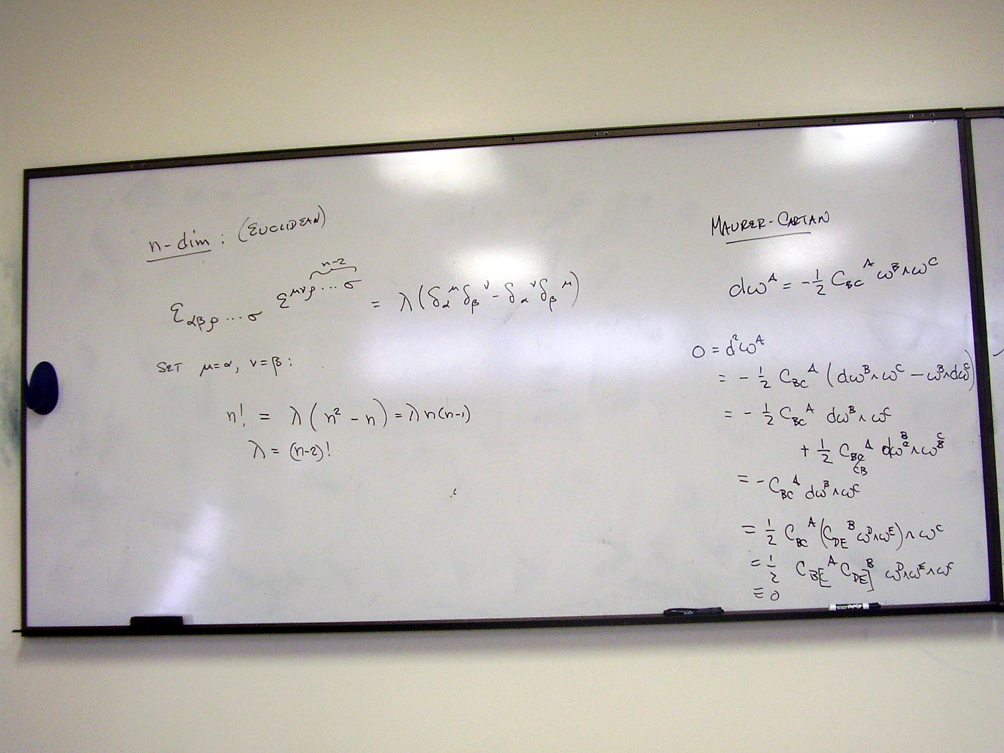
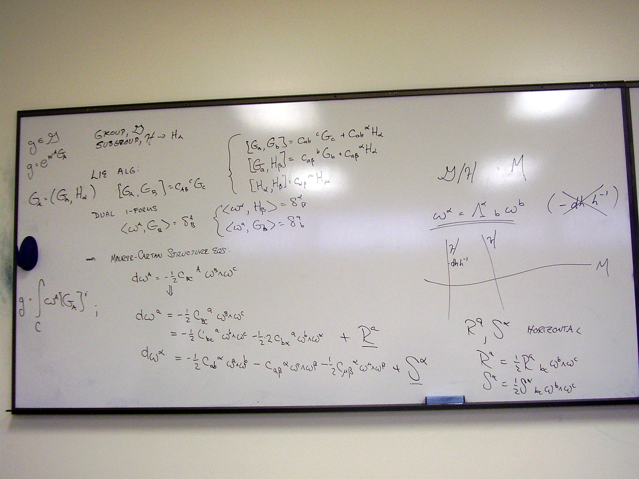
Exercises. Derivation of
the Maurer-Cartan structure equations: The generators of a Lie algebra are
vectors; define 1-forms dual to these vectors and rewrite the commutation
relations in terms of them.
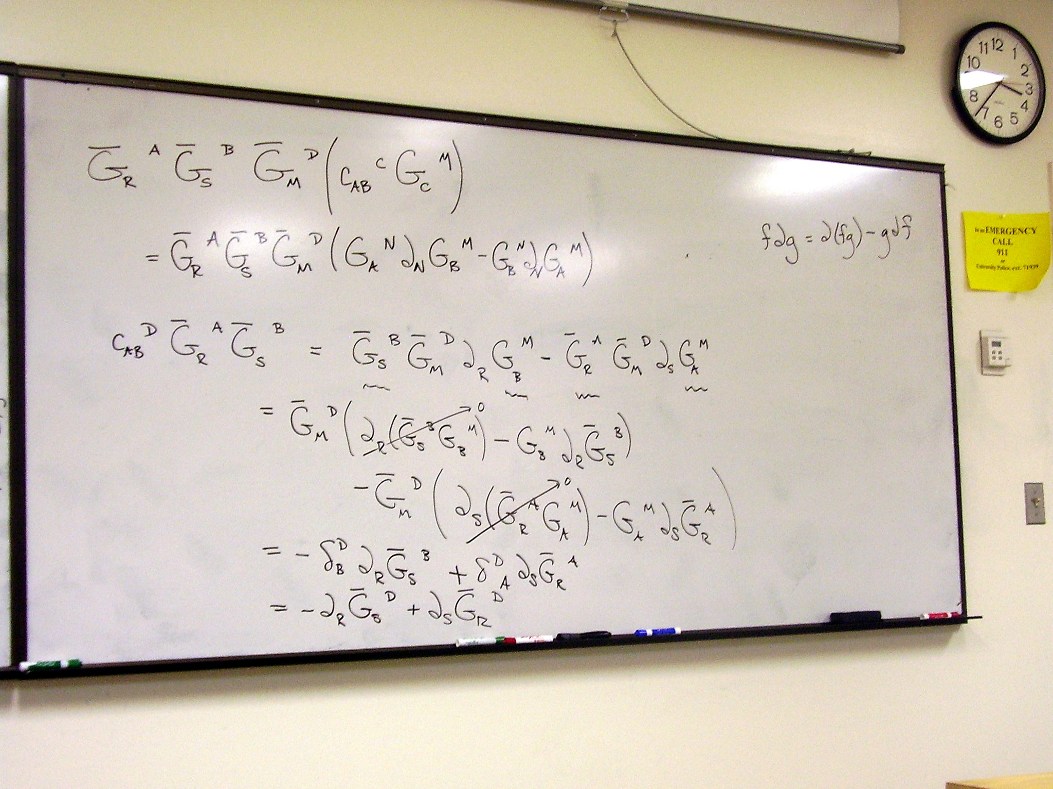
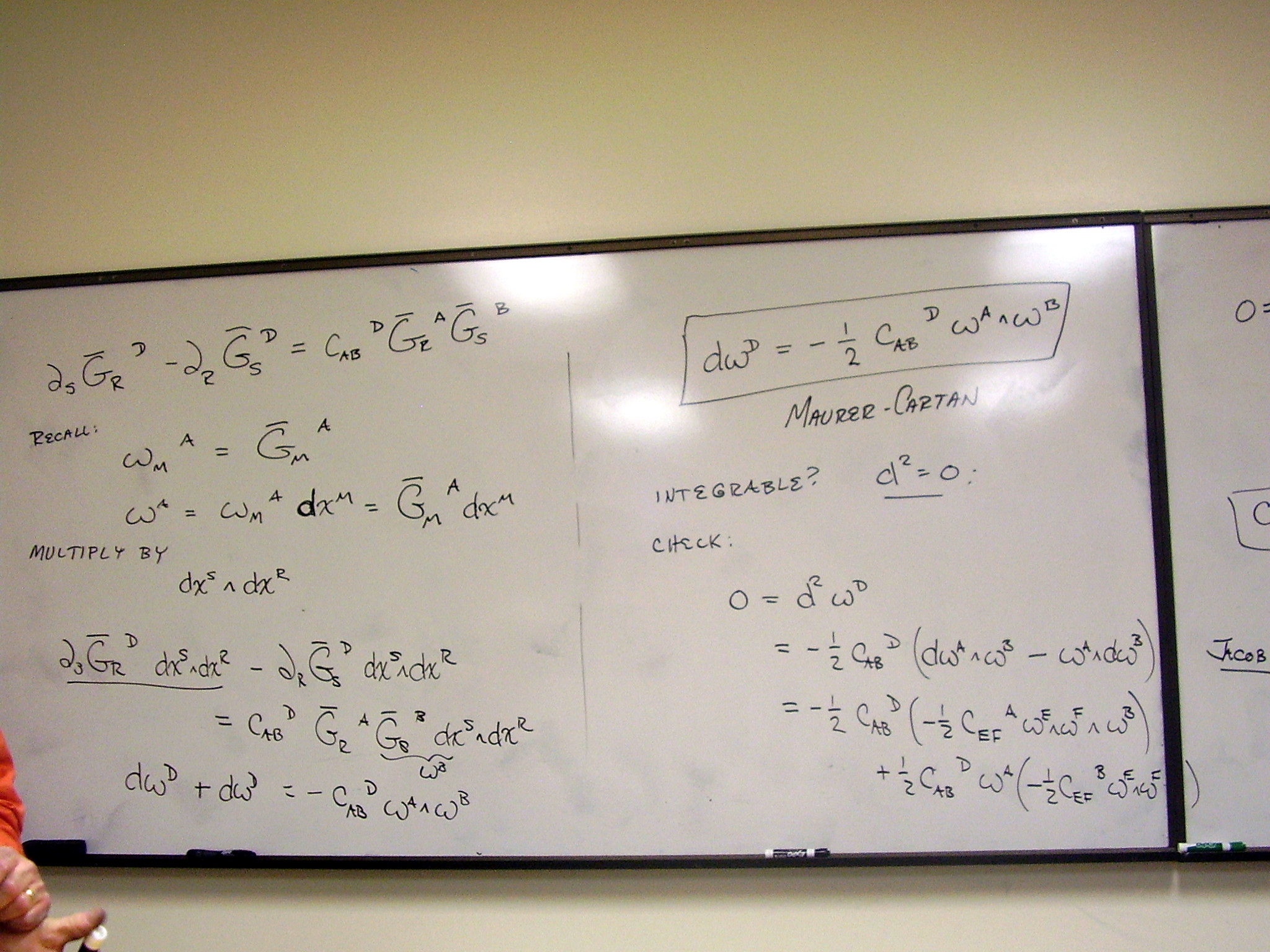
Check integrability; it is
equivalent to the Jacobi identity. (Starts on previous slide)
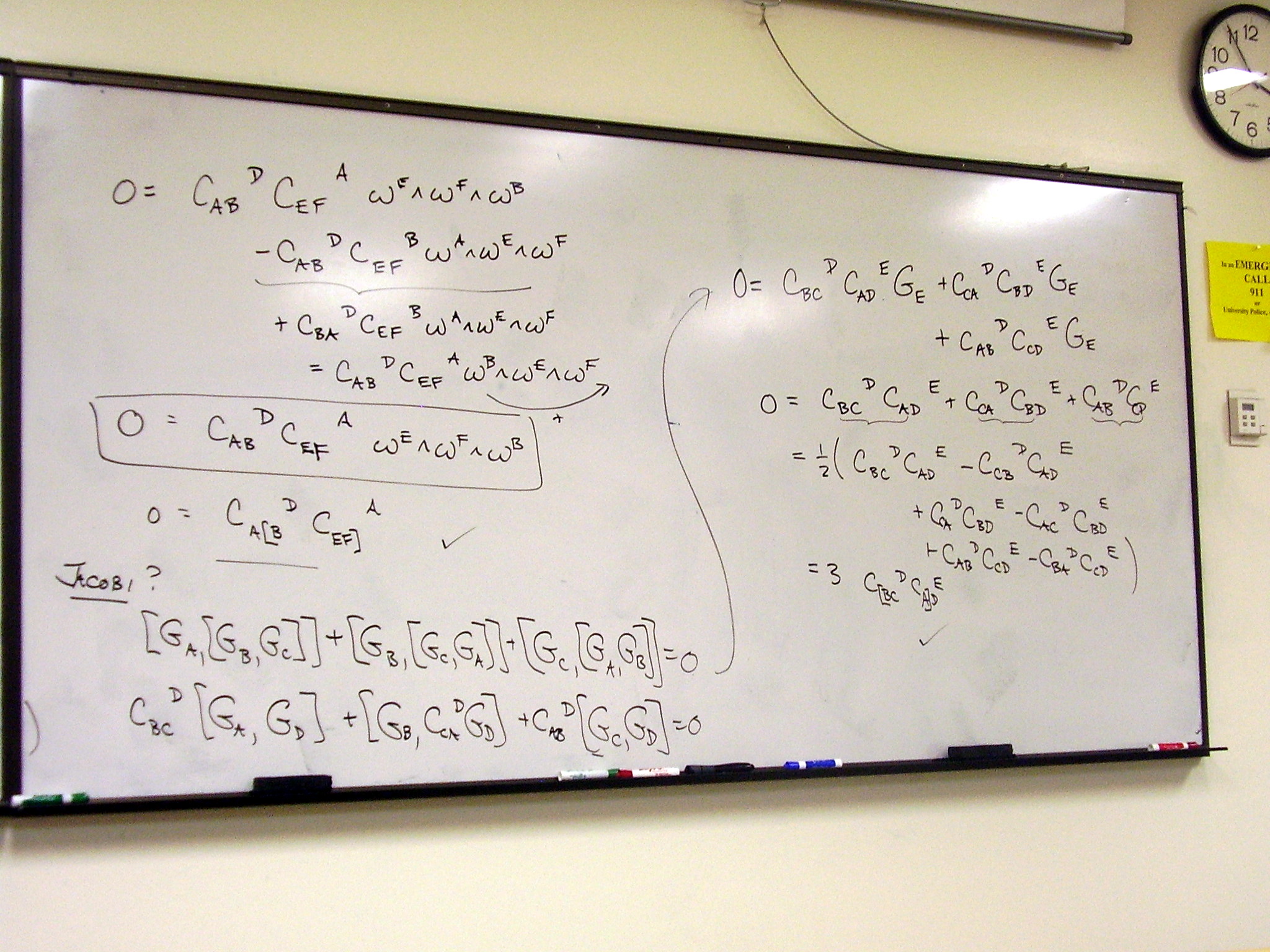
Examples: SO(2); SL(2,C)
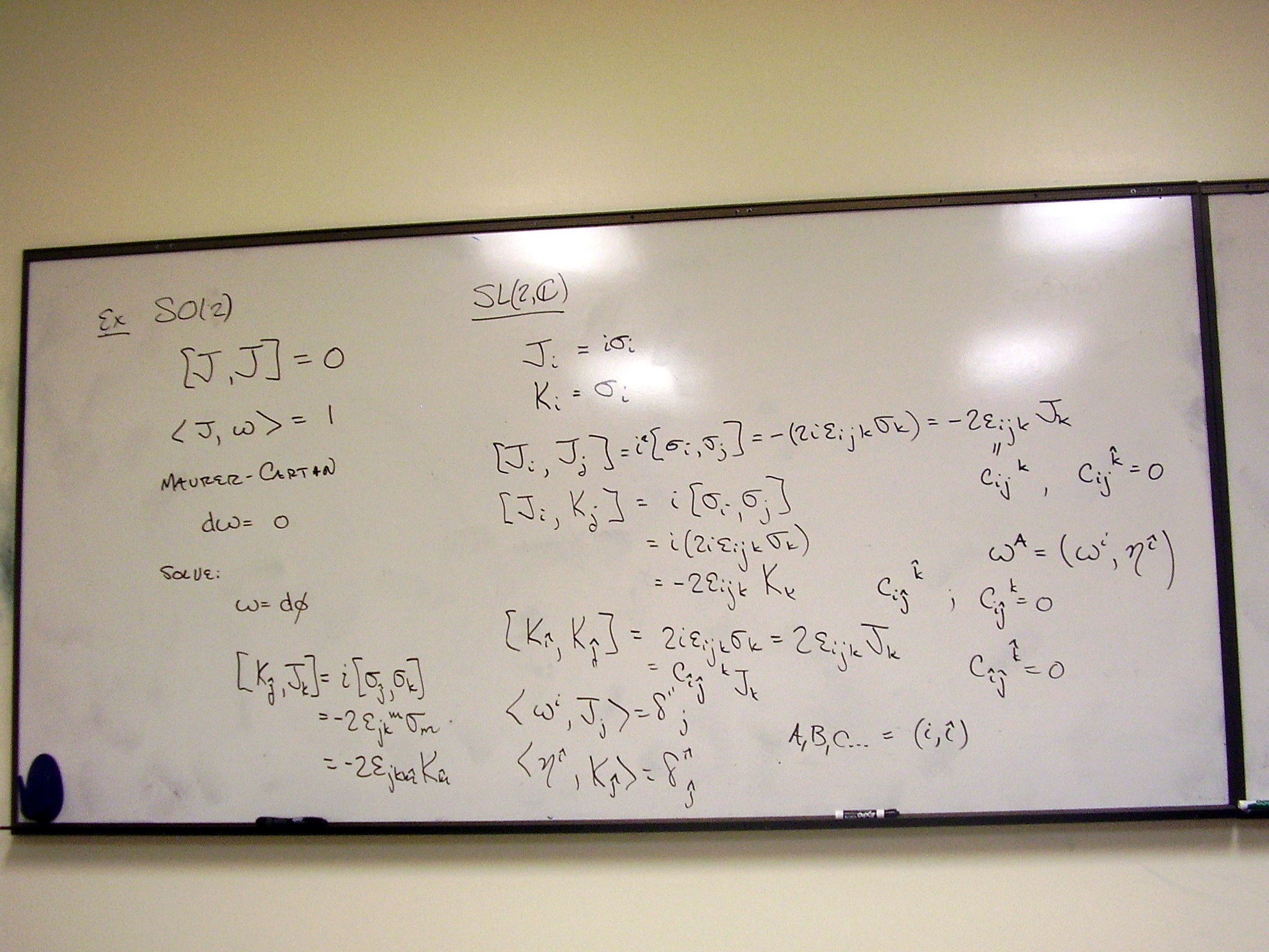
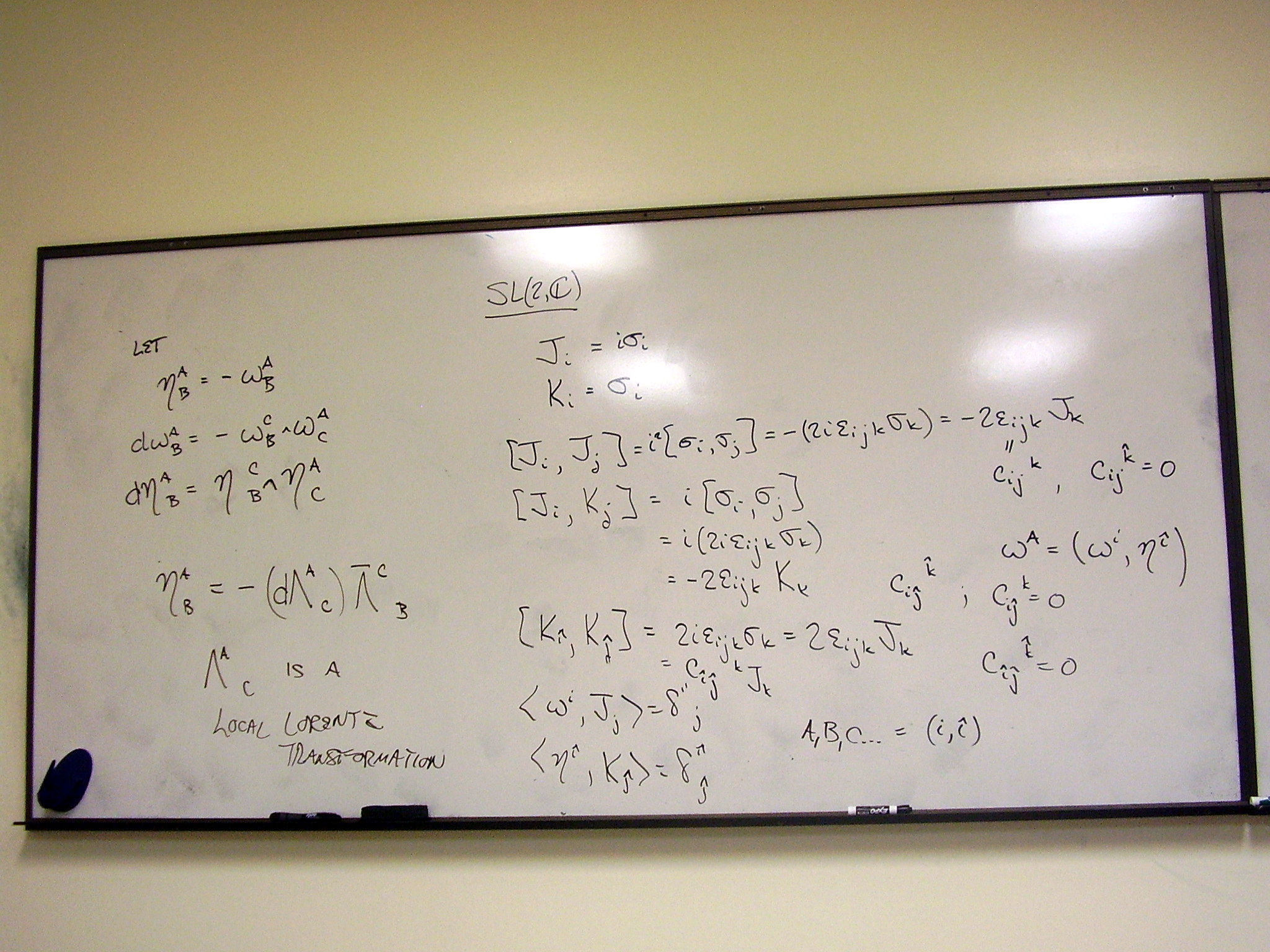
Friday, February 20,
2009
Lecture:
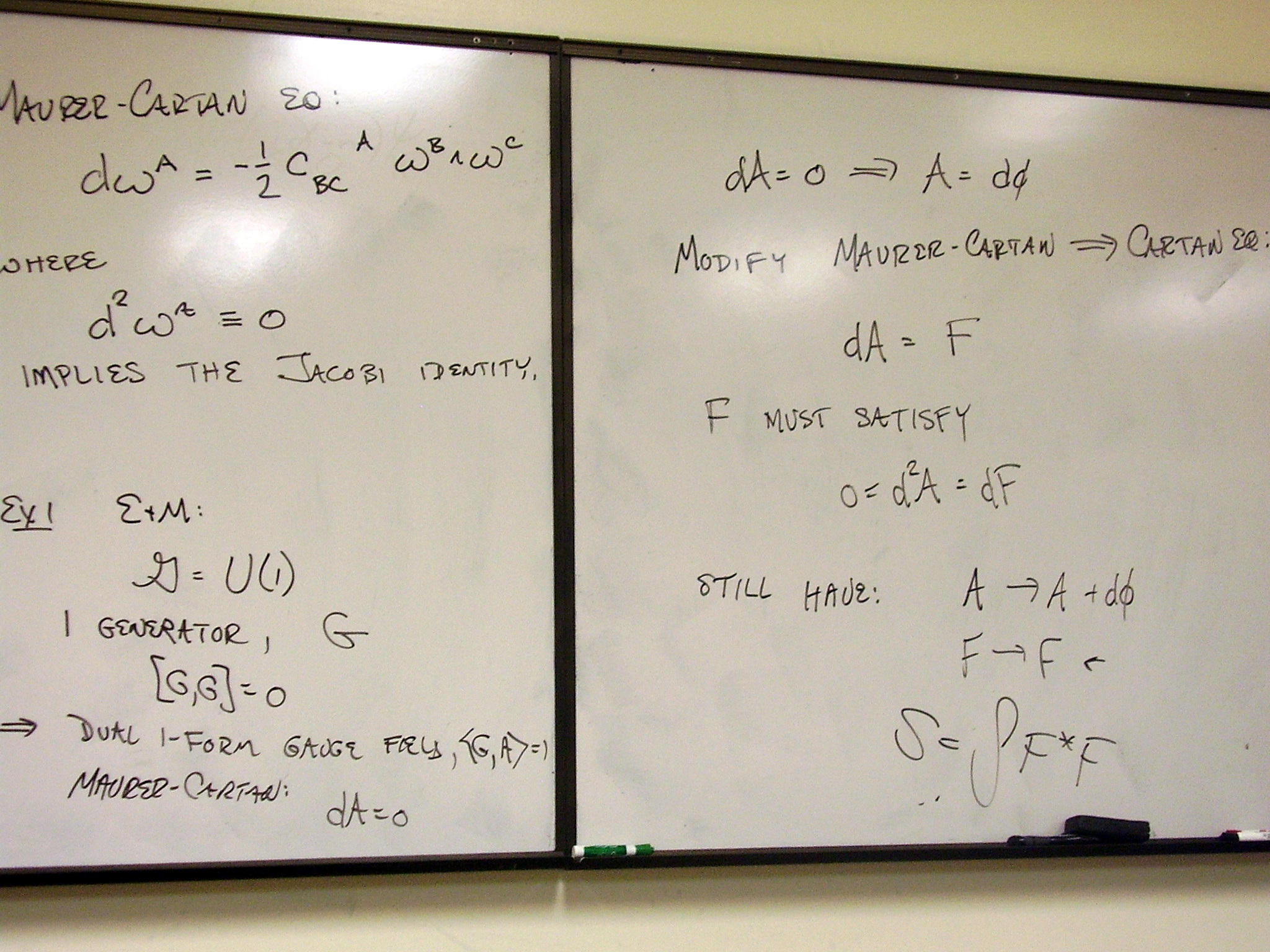
The Cartan structure equations: gauging the Maurer-Cartan equations
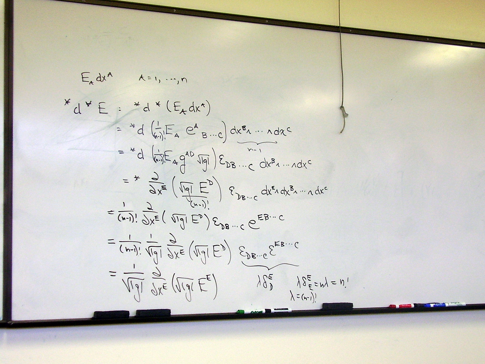
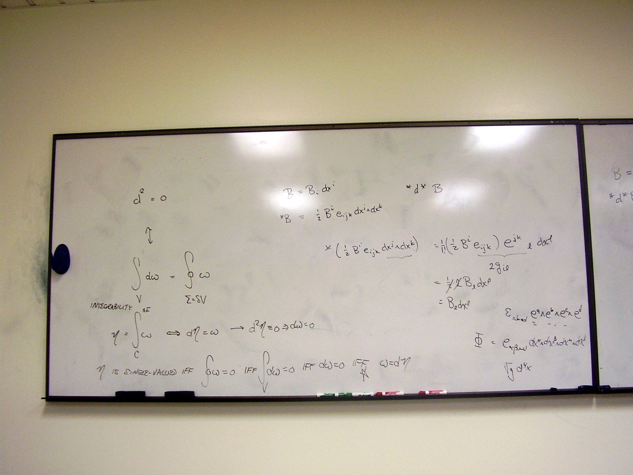
The divergence theorem using
differential forms:
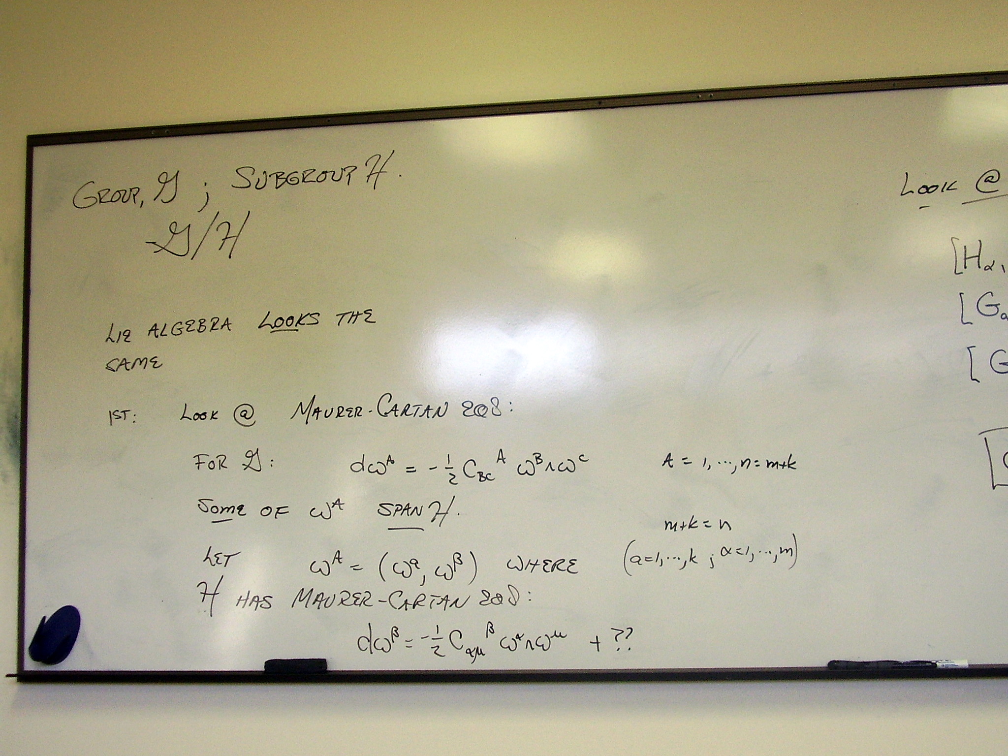
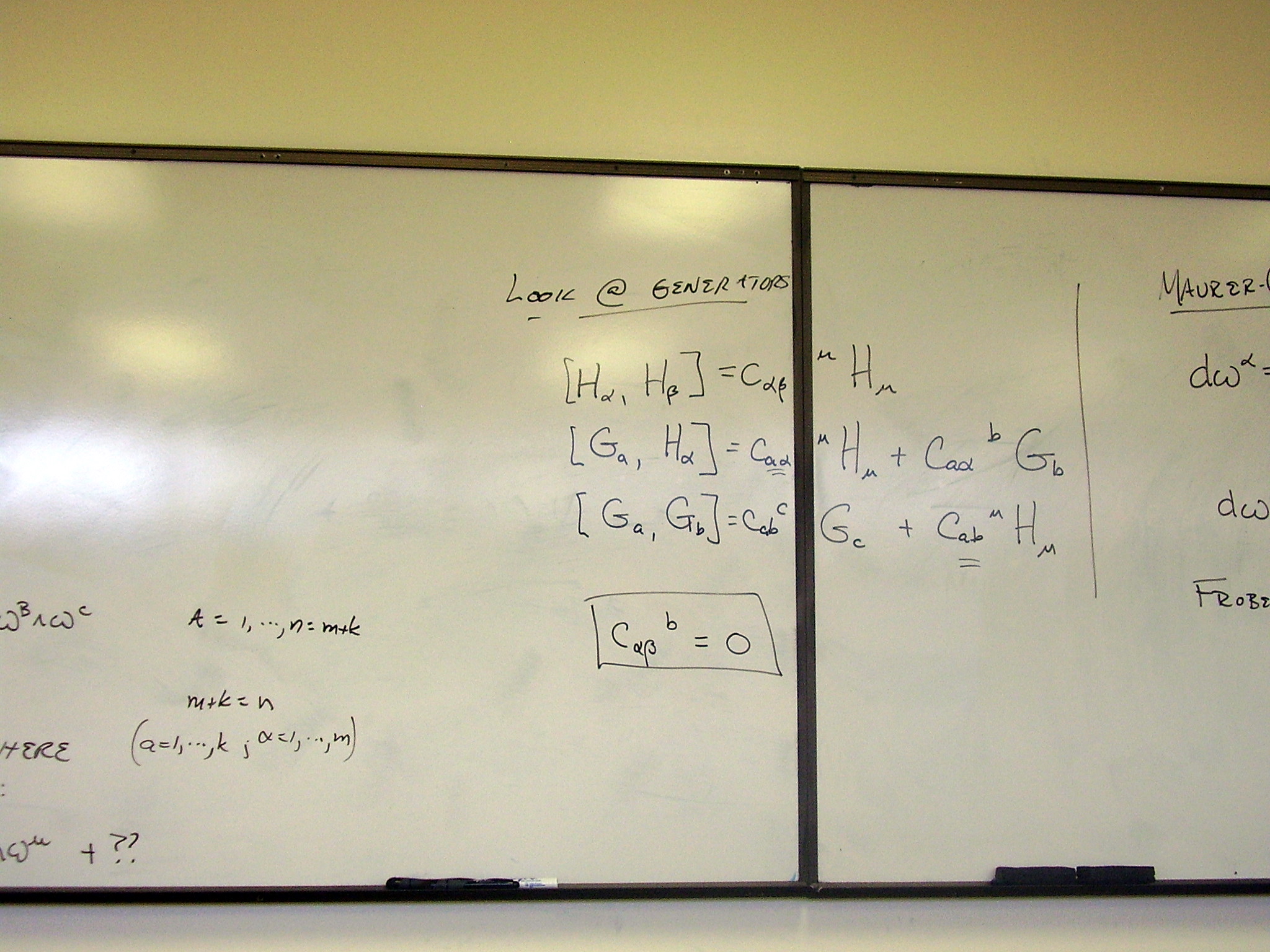
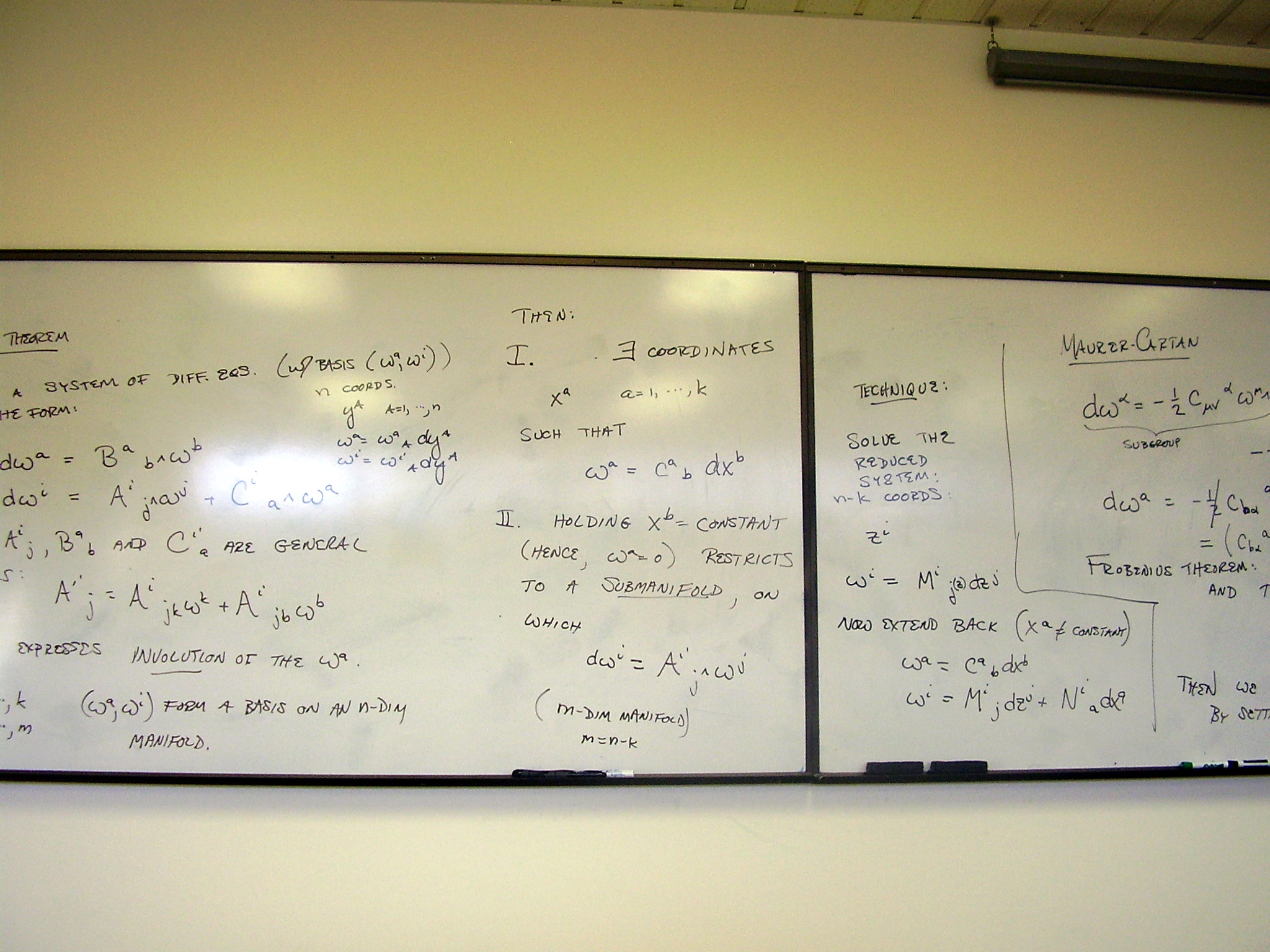
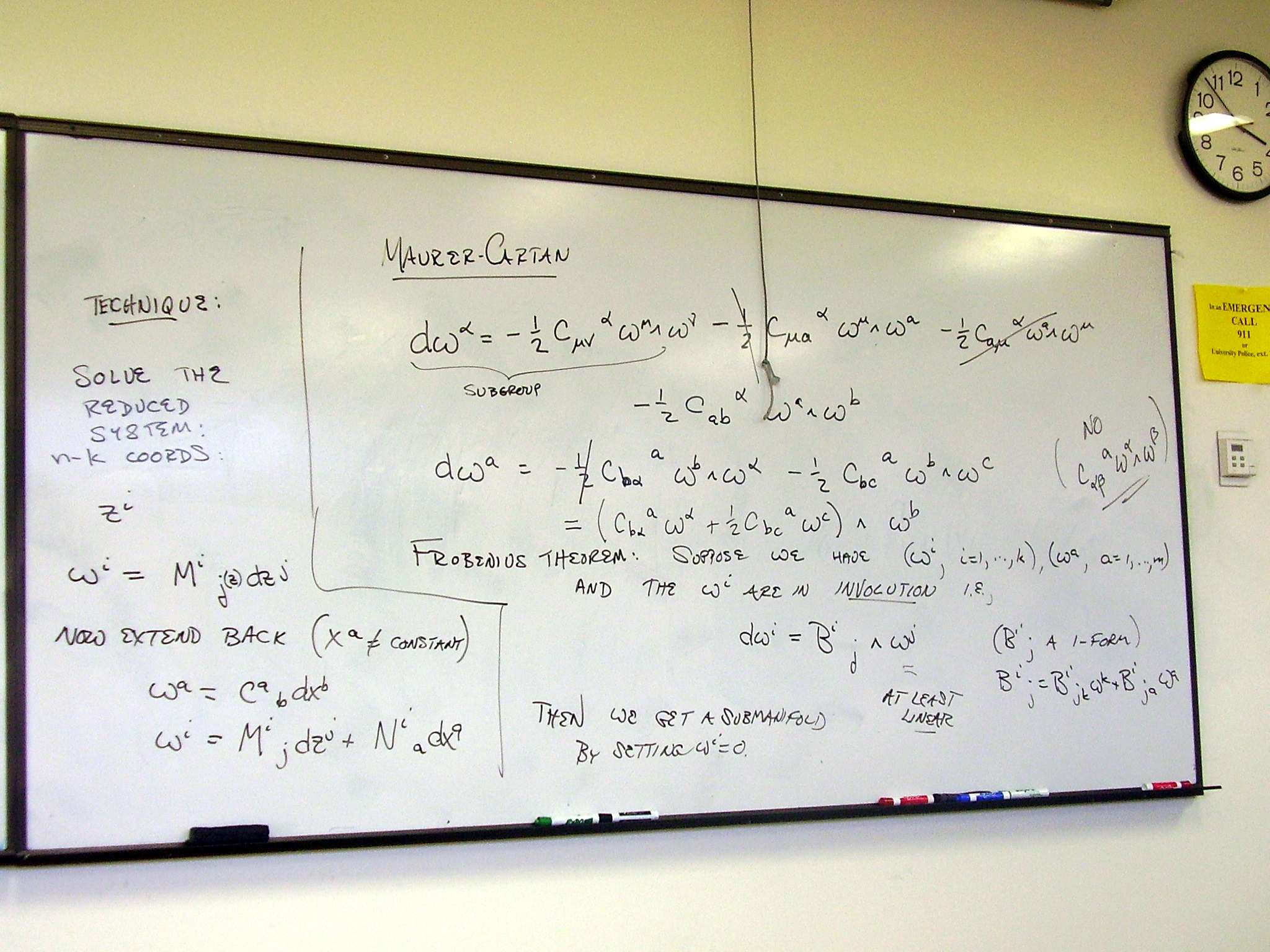
The effect of taking a group
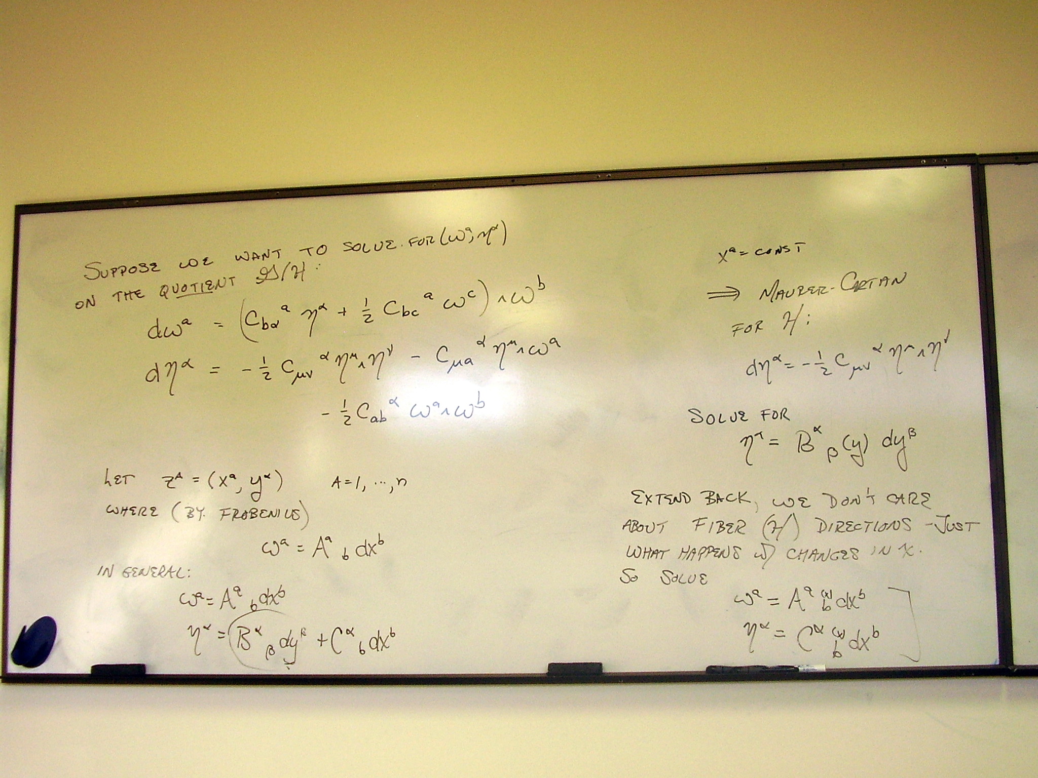
quotient on the Maurer-Cartan equations. How do we identify a Lie subgroup
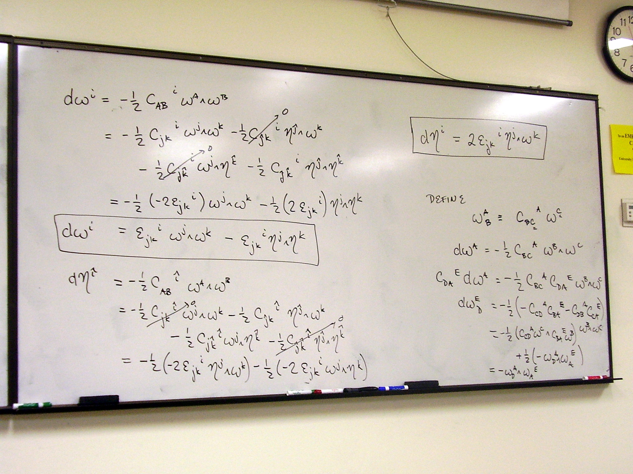
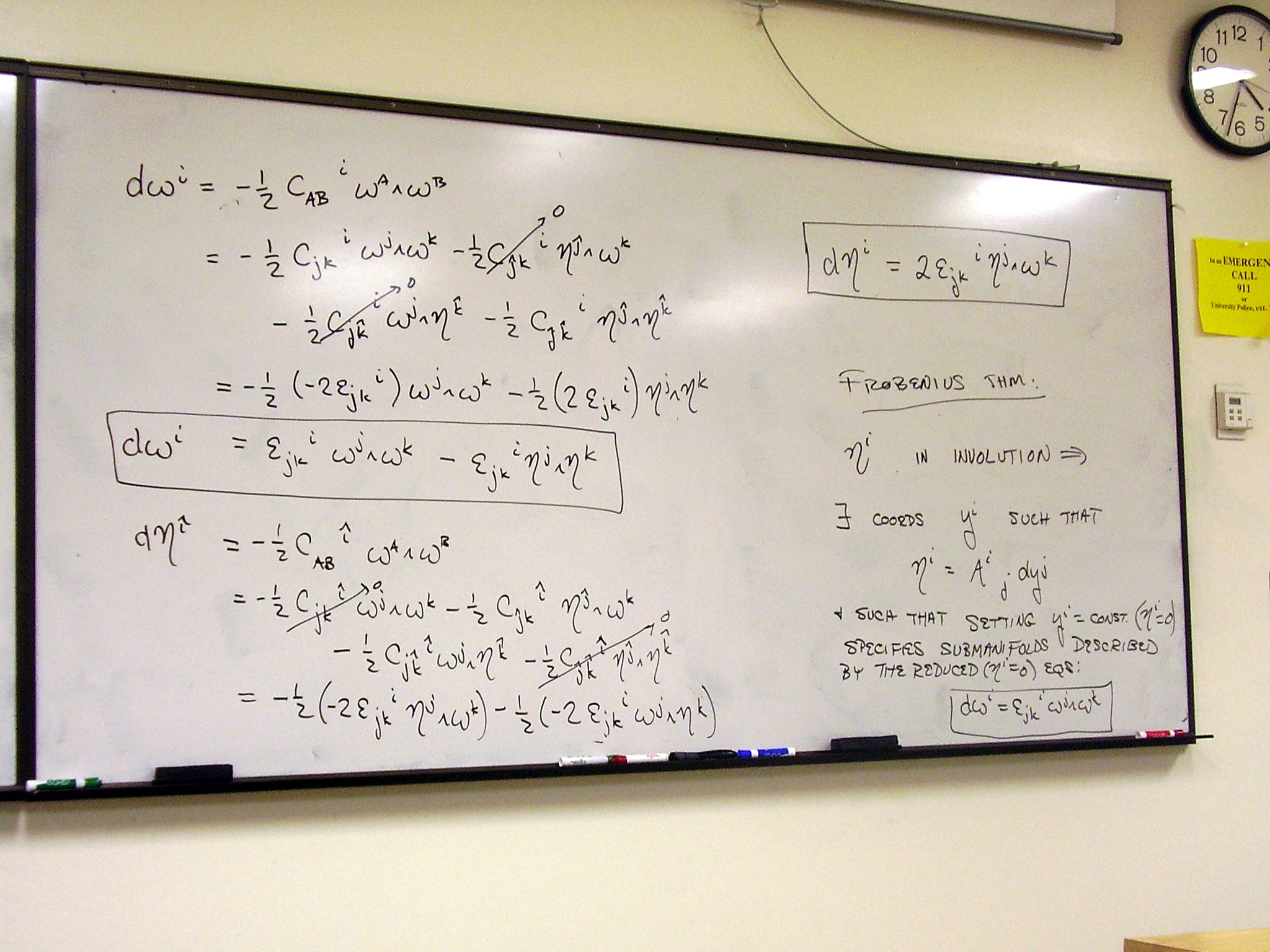
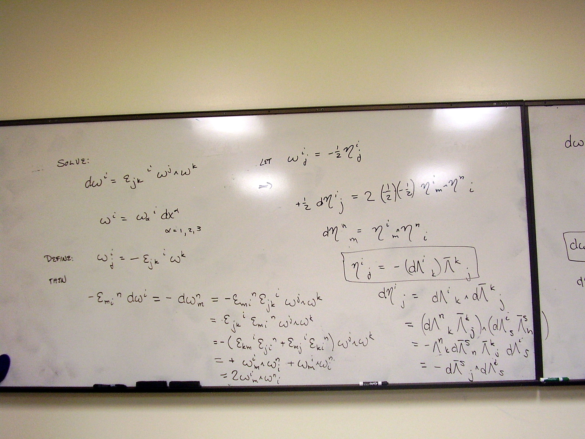
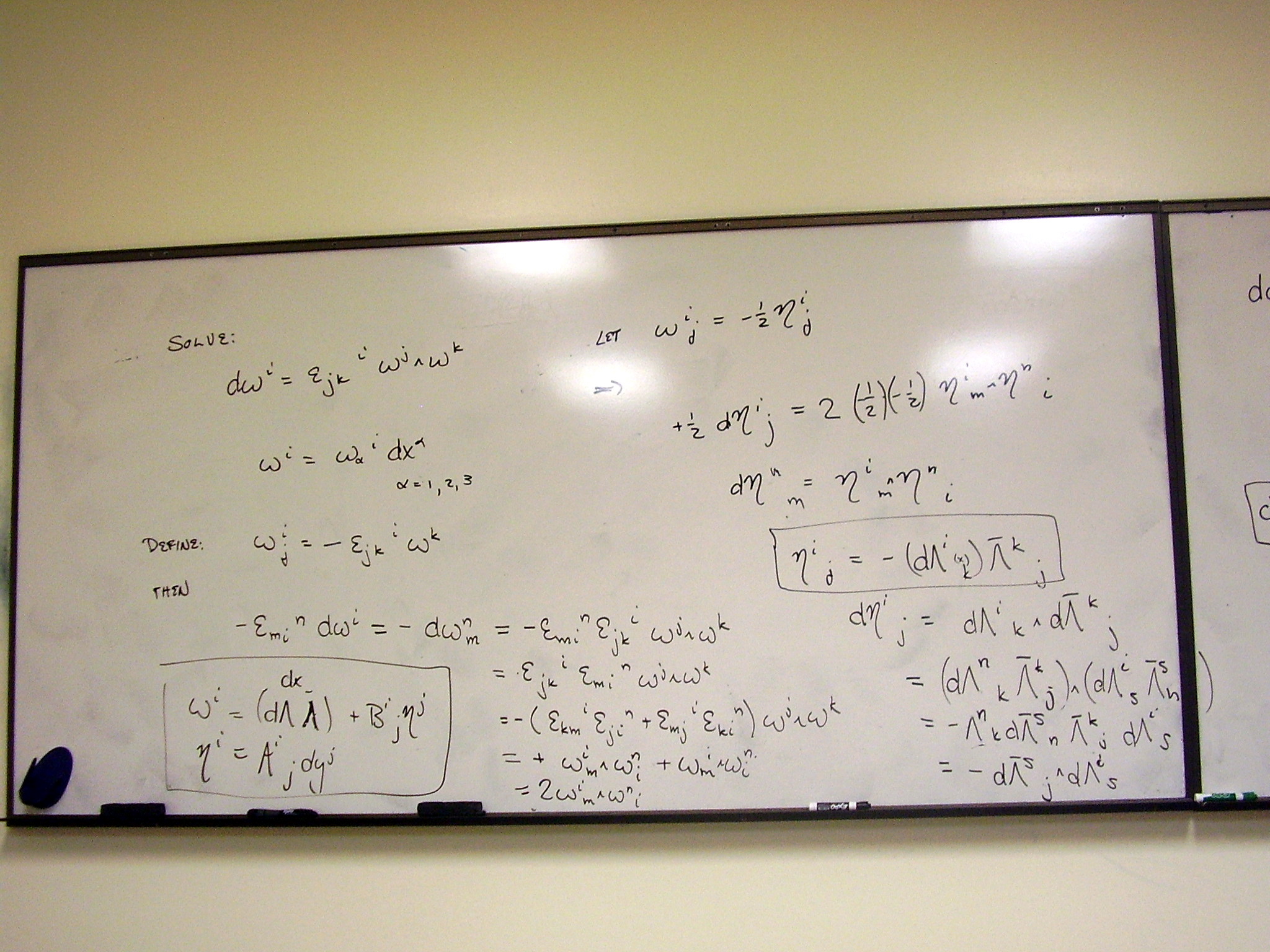
using the Maurer-Cartan equations? The Frobenius theorem. (Some duplicate
slides)
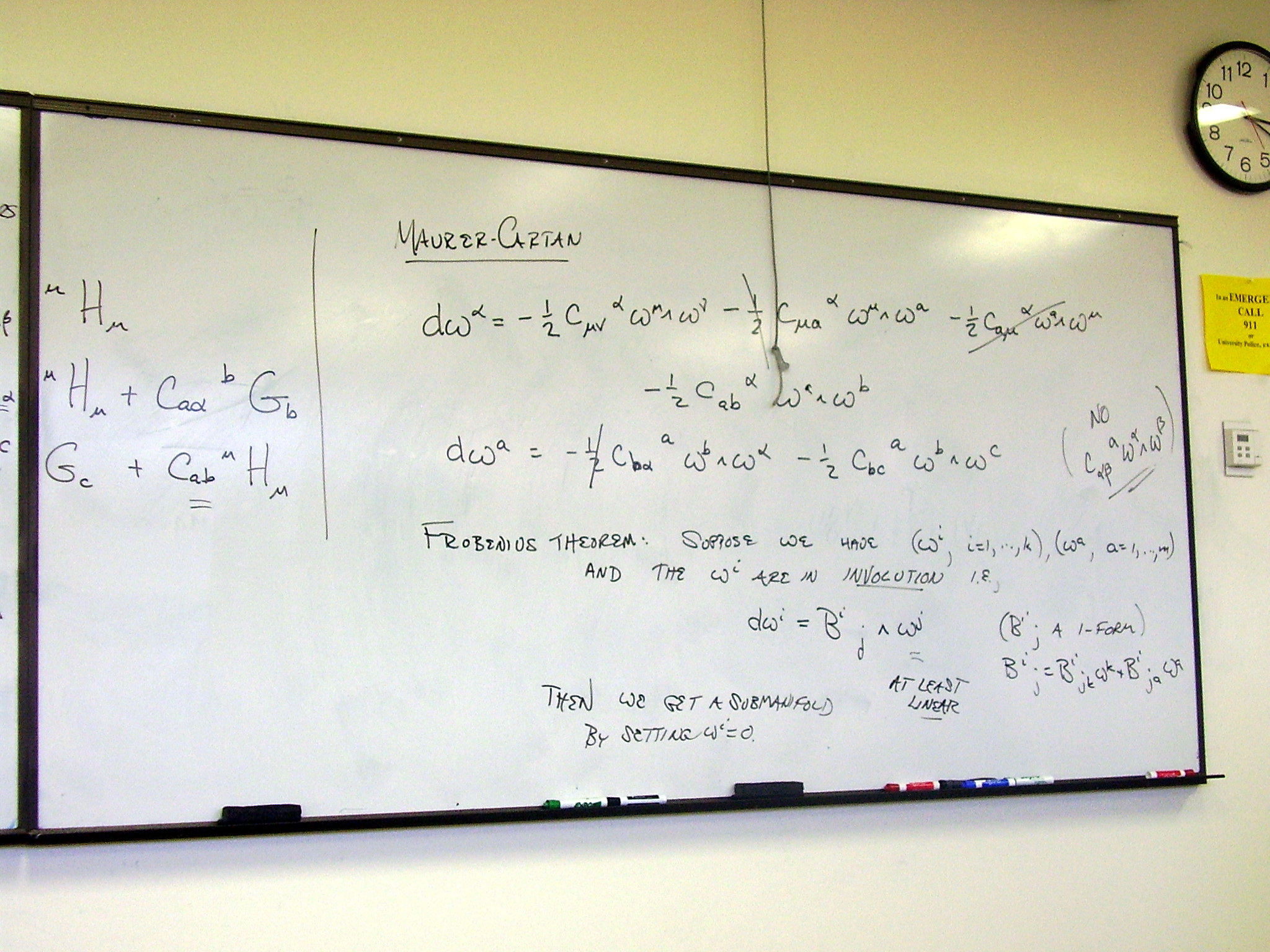
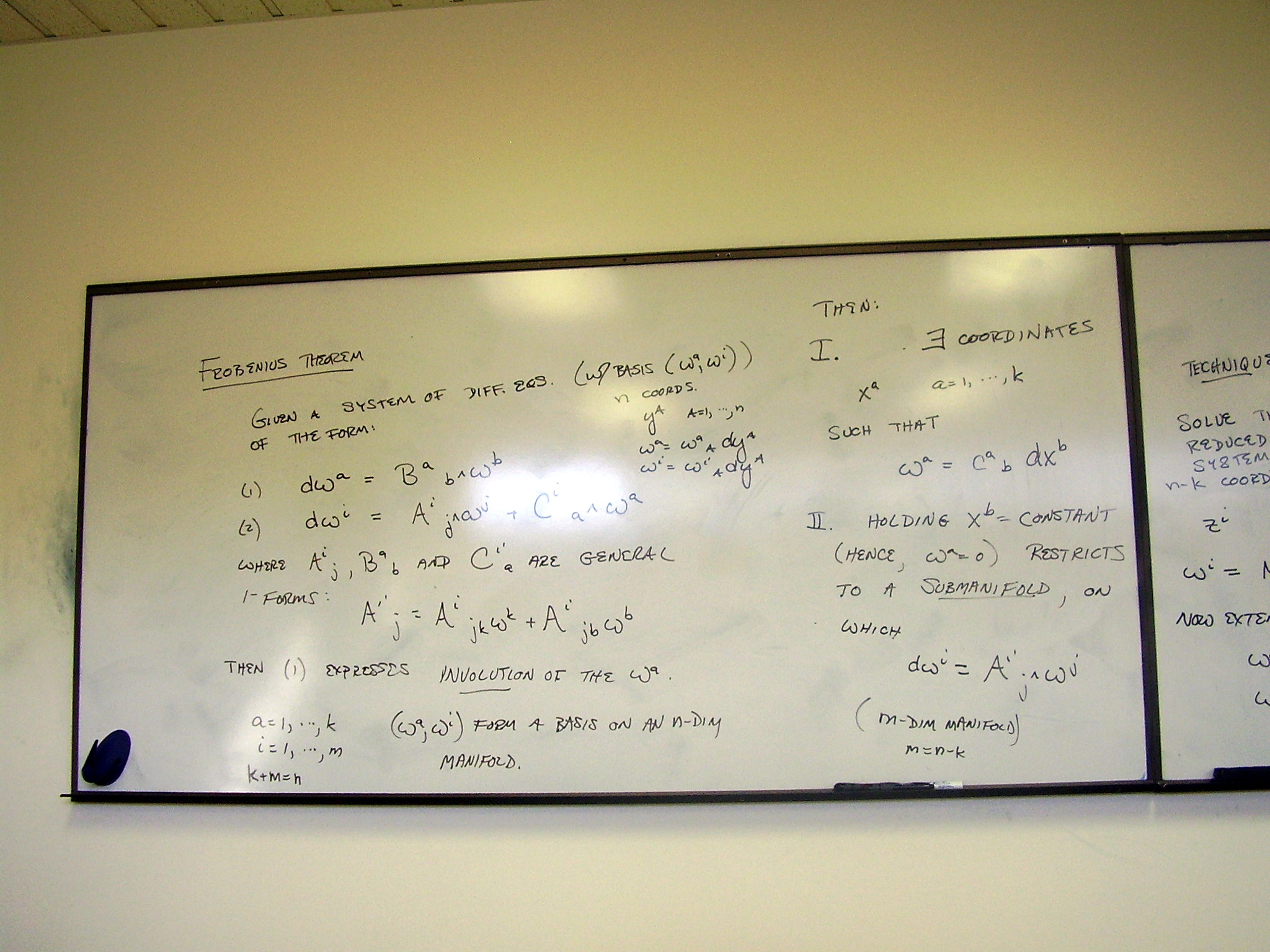
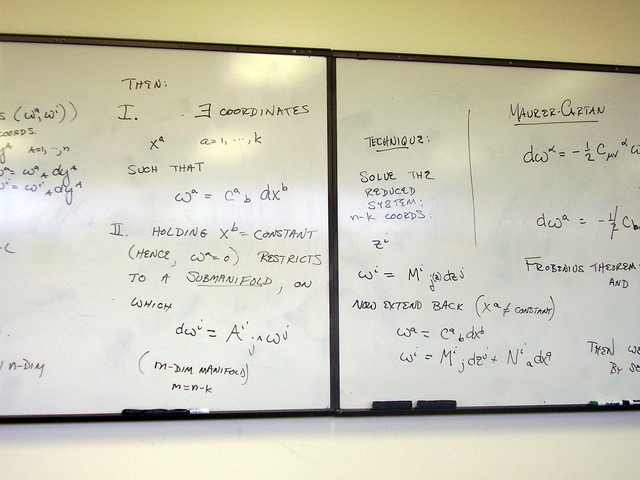
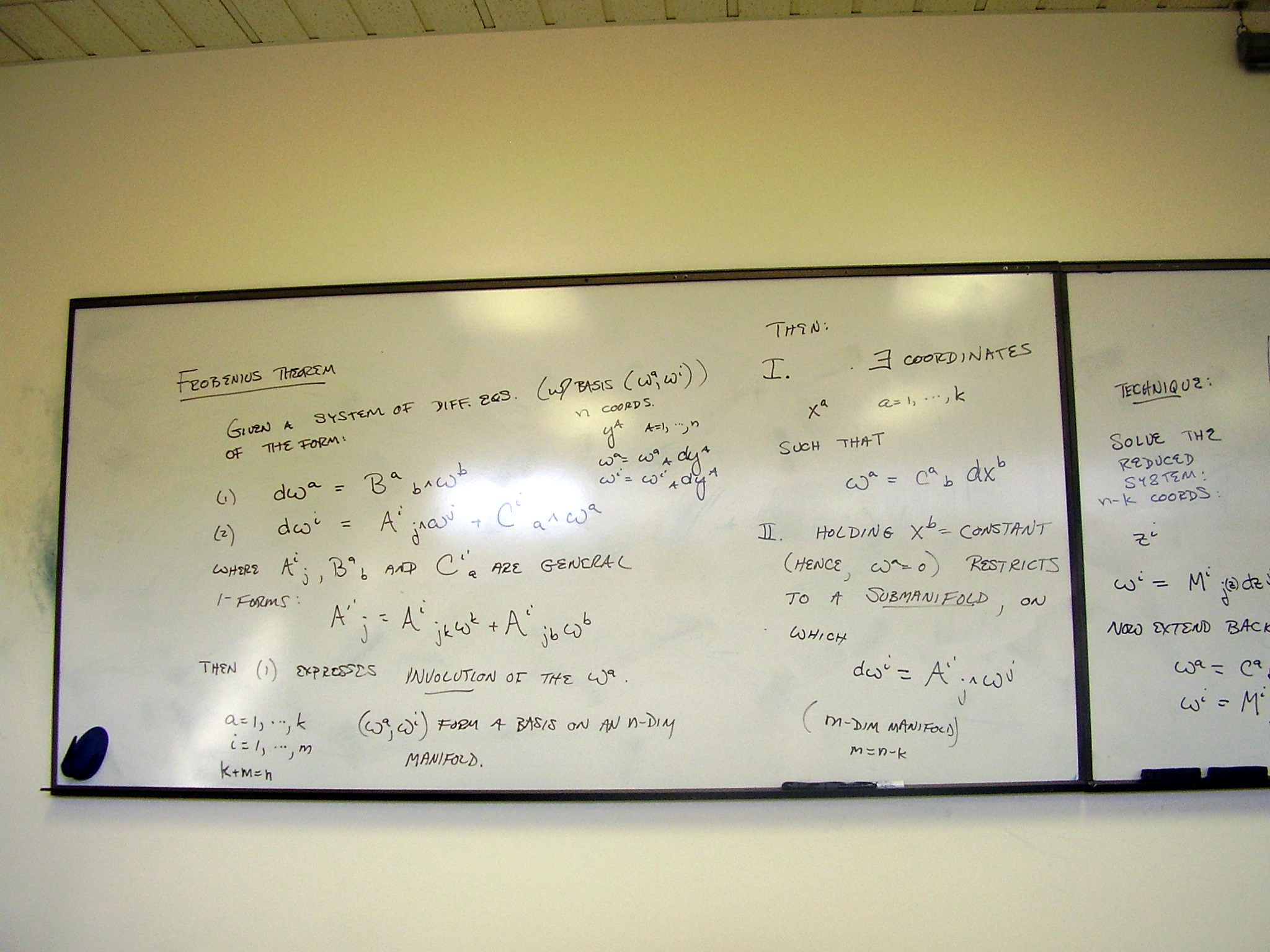
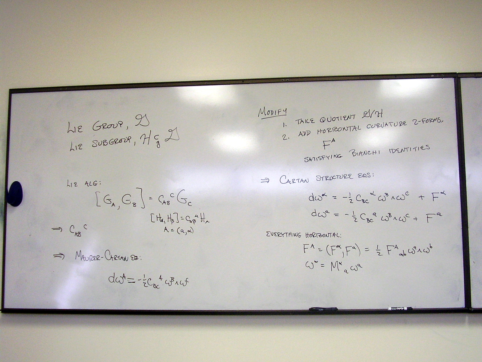
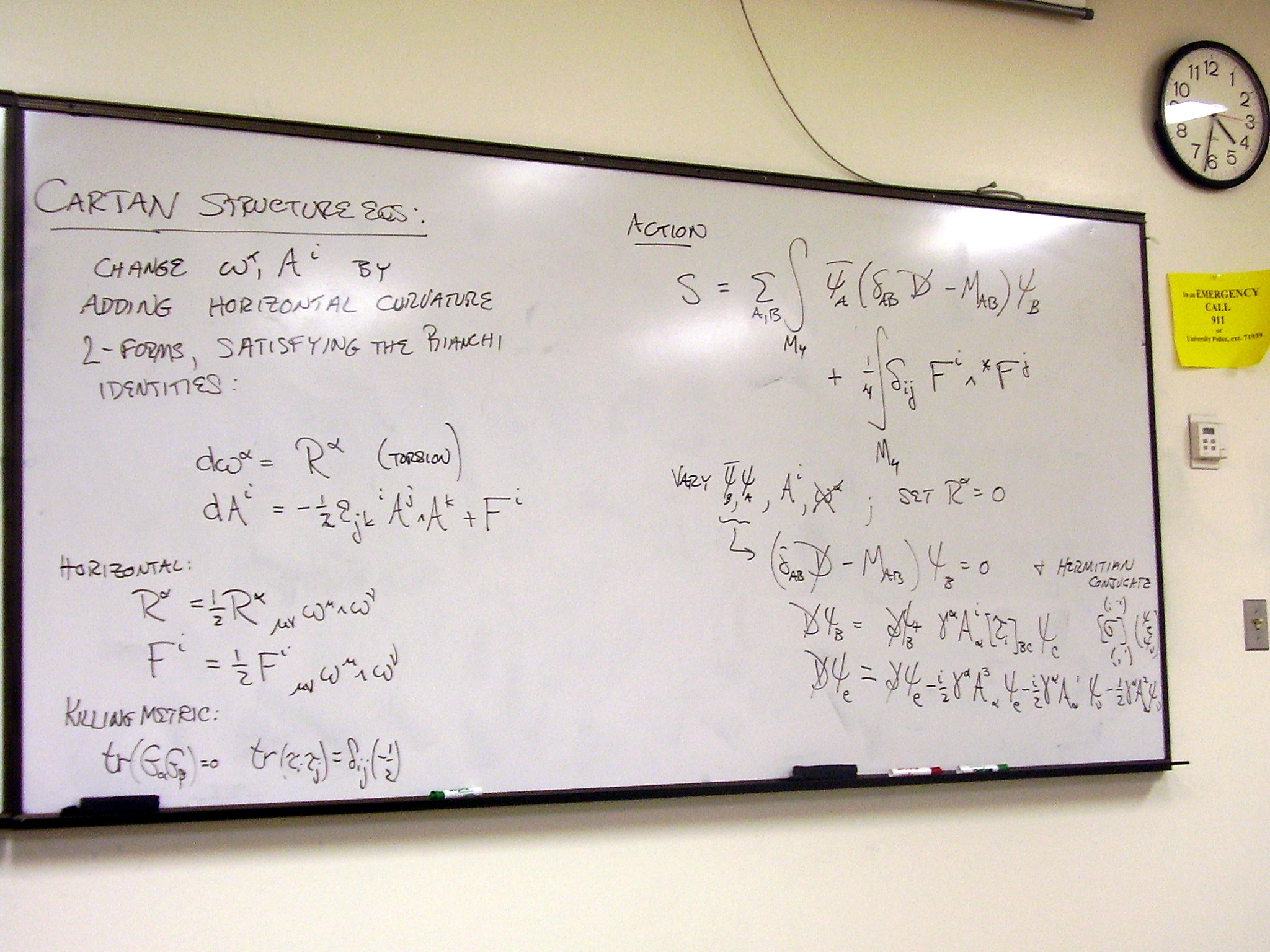
Example: SL(2,C)
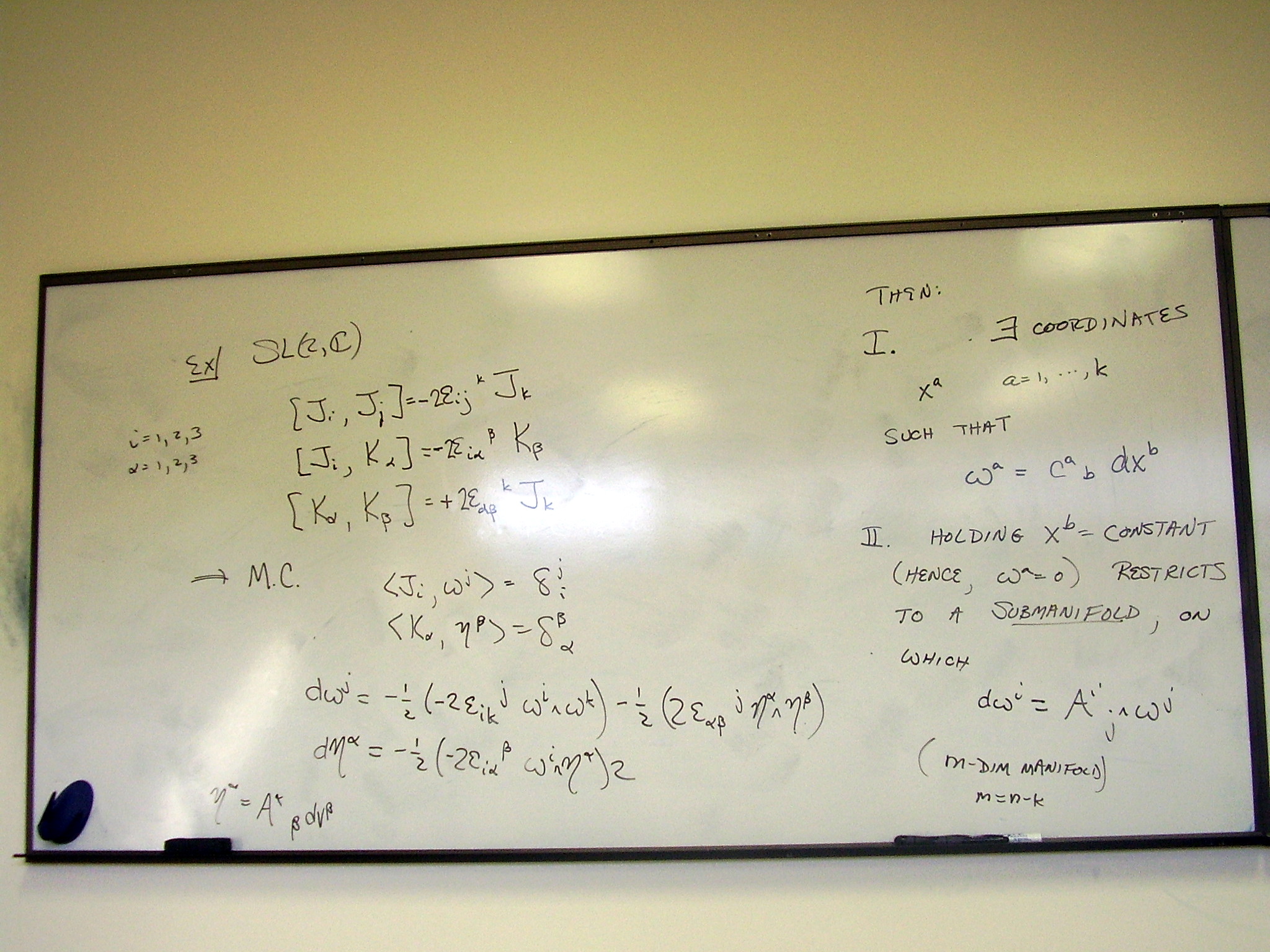
Generalizing the
Maurer-Cartan structure equations. Changing the connection changes each
structure equation by a 2-form. Requiring these 2-forms to be horizontal leaves
the subgroup of the quotient as a symmetry; the curvature 2-forms then describe
the base manifold of the quotient.
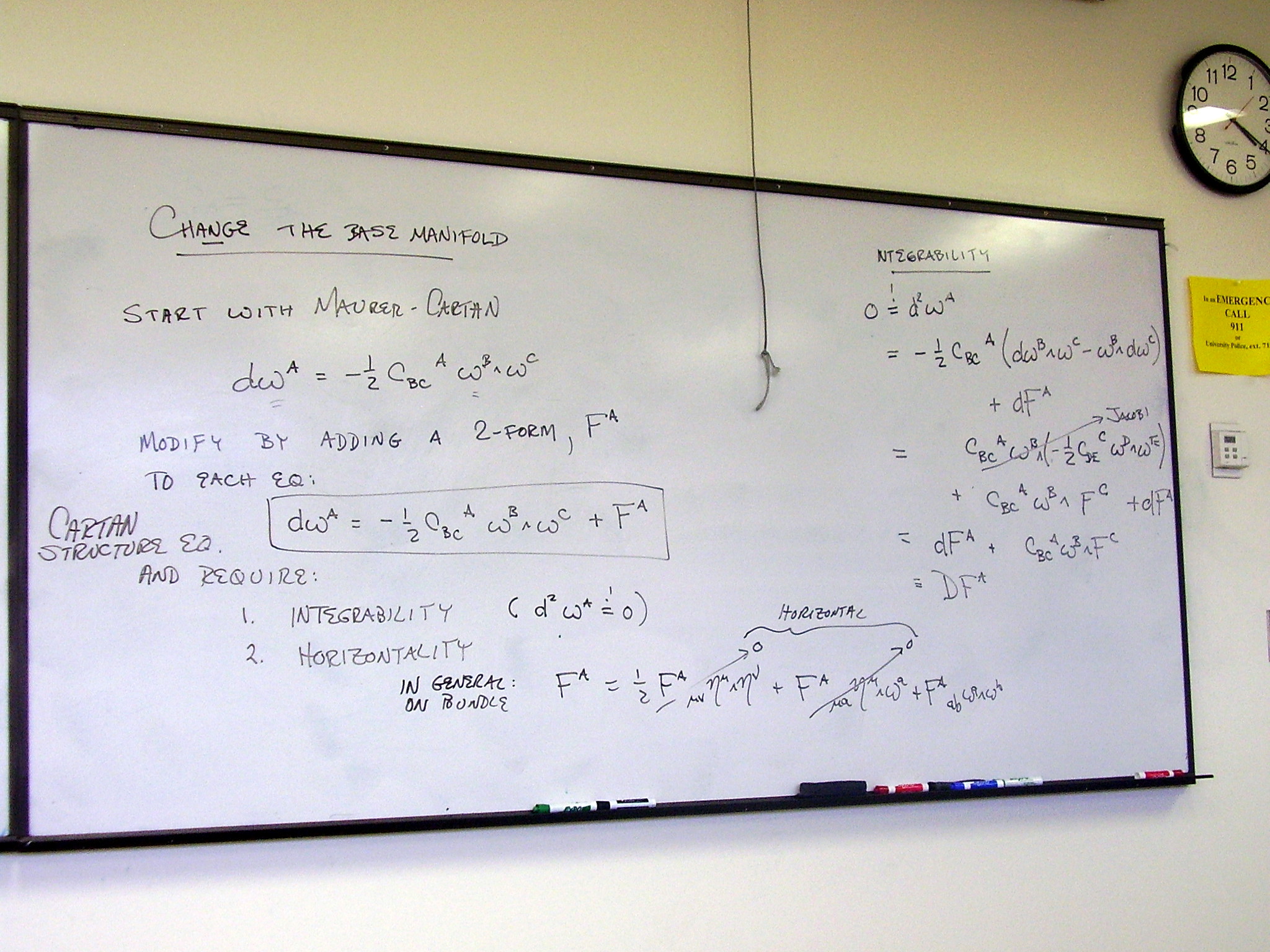
The curvature 2-forms we
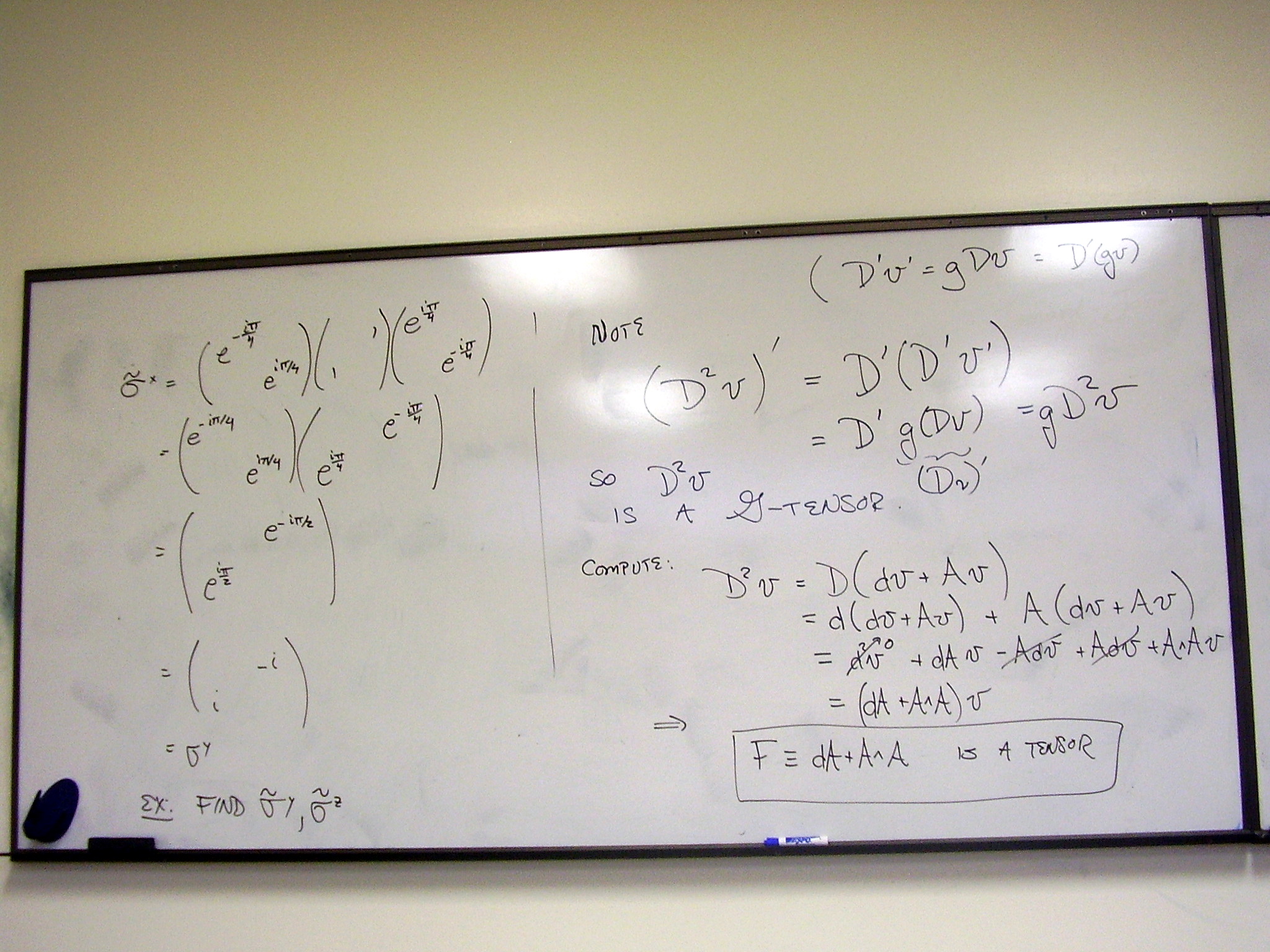
have added are tensors with respect to local group transformations.
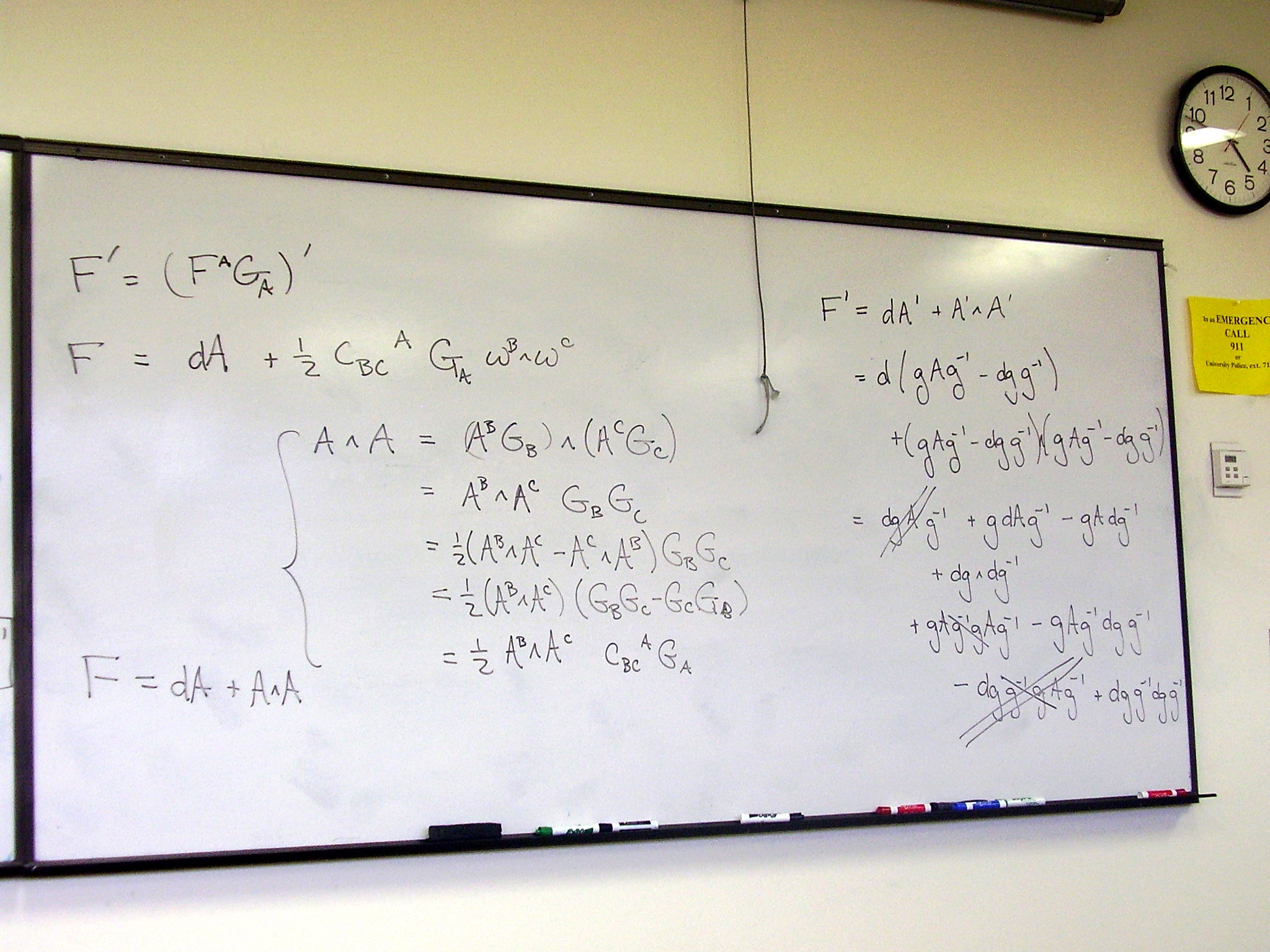
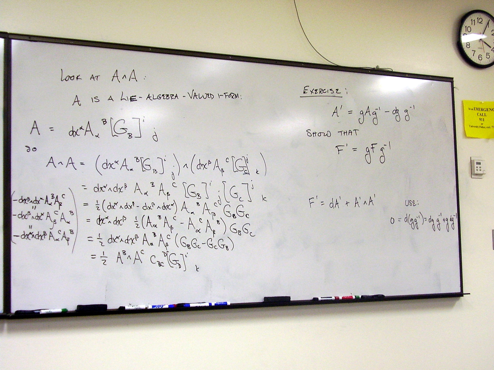
Exercises:
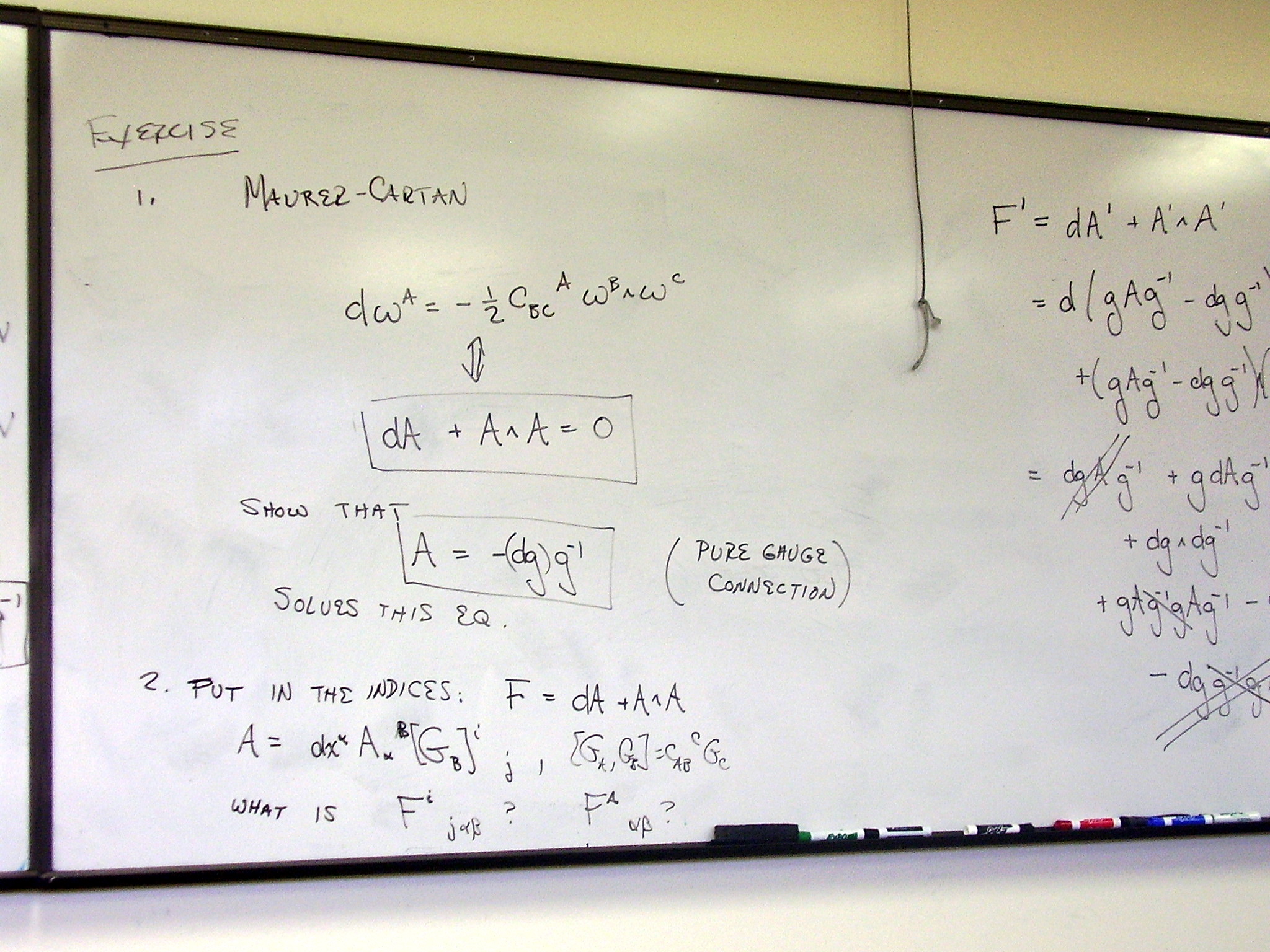
Vicious dento-quantized
shark:
Monday, February 23,
2009
Lecture:
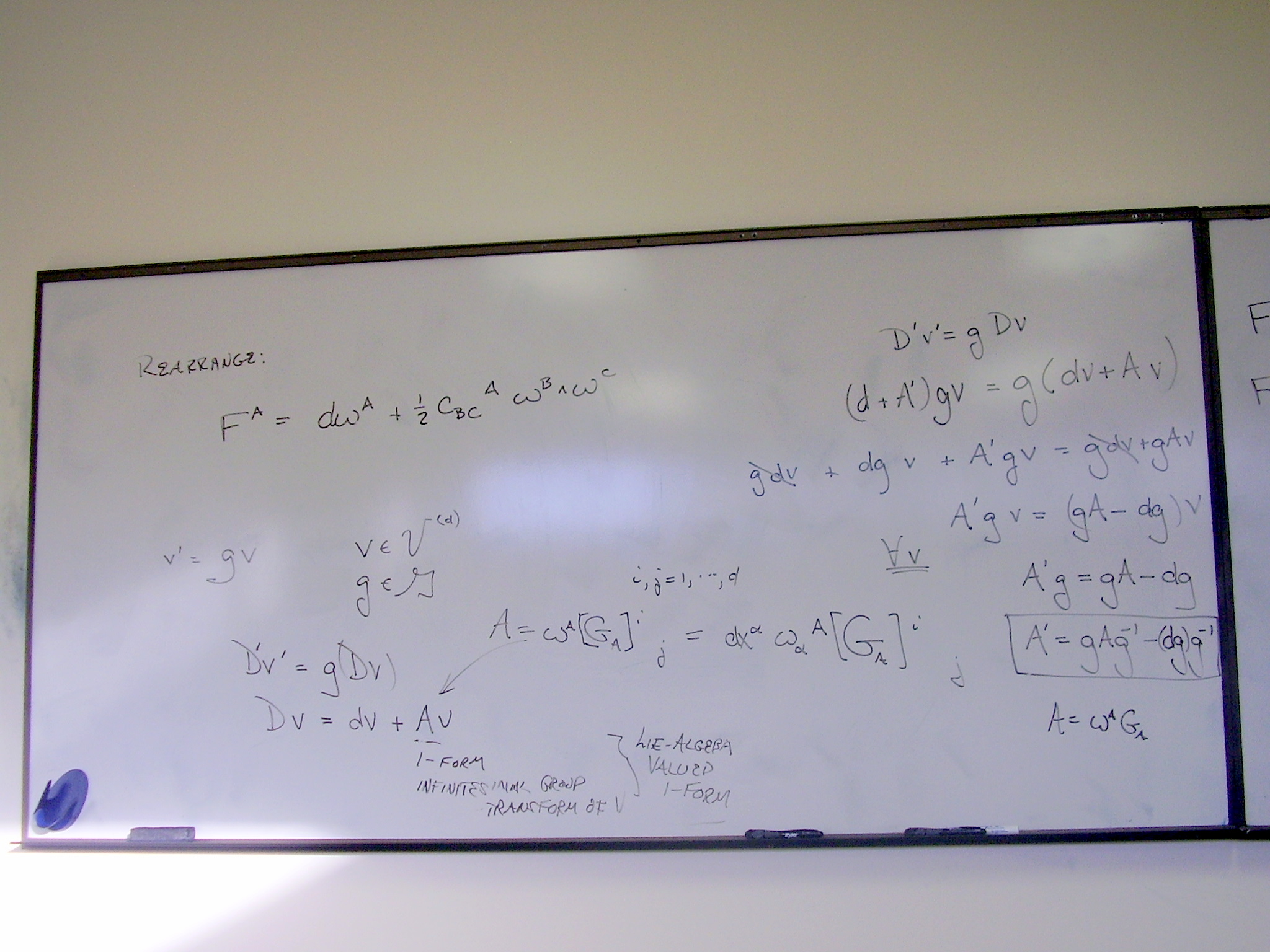
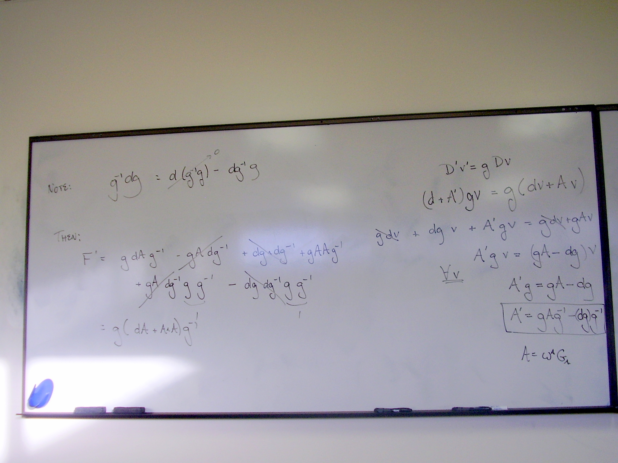
The gauge-covariant derivative; covariance of the curvatures
The dual 1-forms of the
Maurer-Cartan equations provide a group-covariant connection. We may define a
covariant derivative. Several things happen at once. The Lie group acts on the
Lie algebra, and the Maurer-Cartan equations determine how the connection
1-forms transform. Their transformations properties are exactly what is
required to make the covariant derivative covariant.
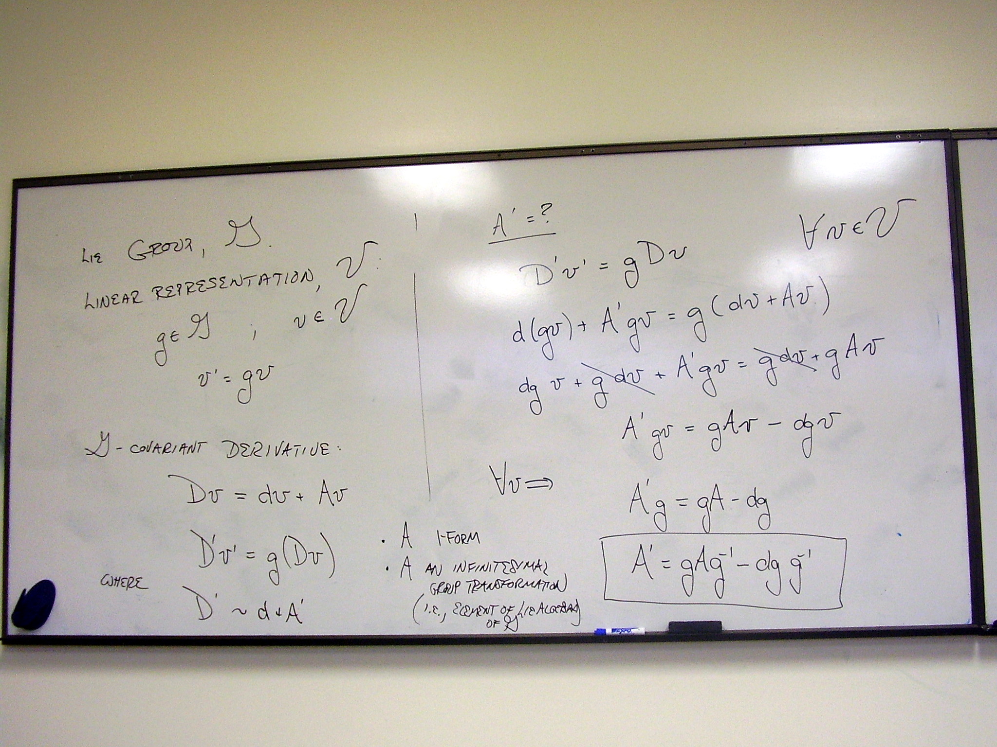
The group acts on the Lie
algebra; an example: SU(2).
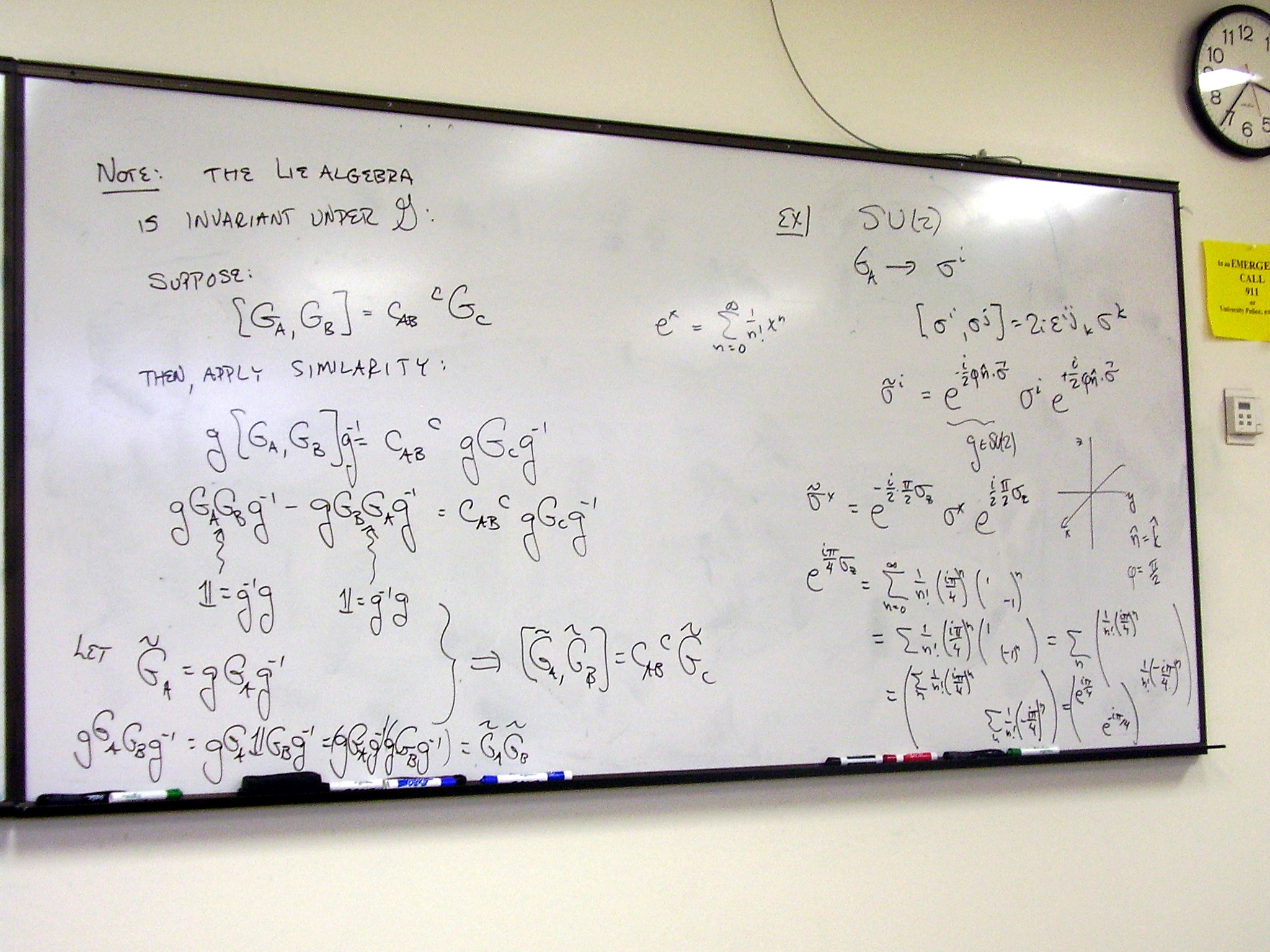
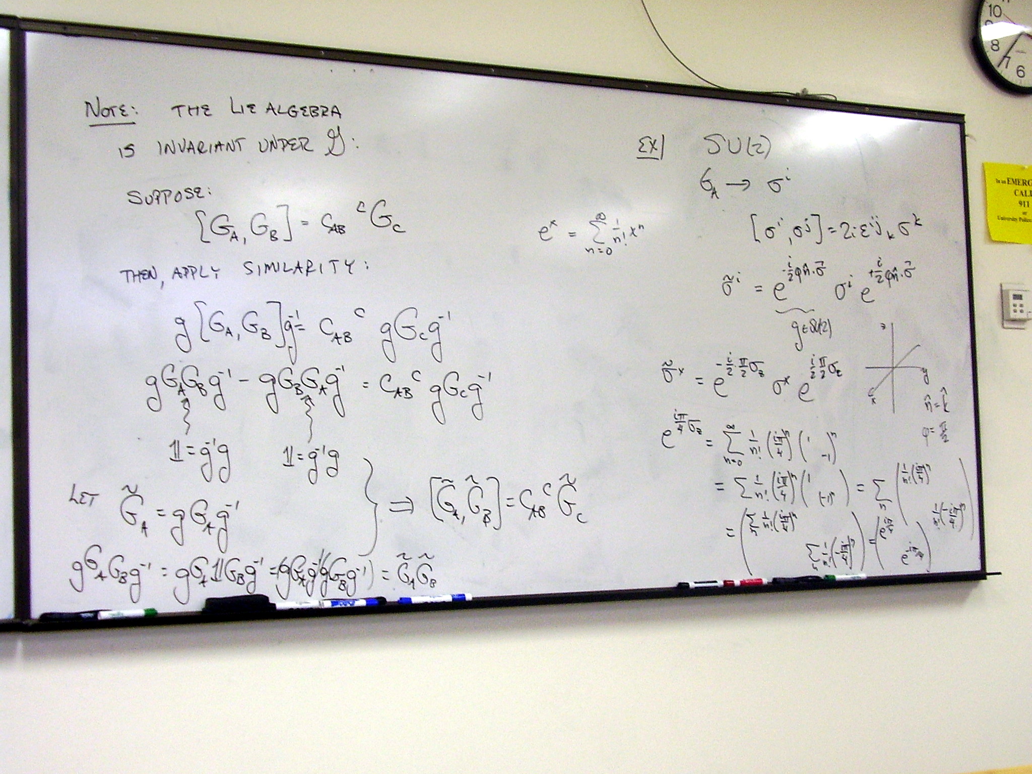
SU(2) example continued; the
curvature constructed using the Ricci identity of the covariant derivative is
the same object we get when we generalize the Maurer-Cartan connection:
Unpacking the connection
1-forms; exercises:
Covariant derivative and
curvature in components:
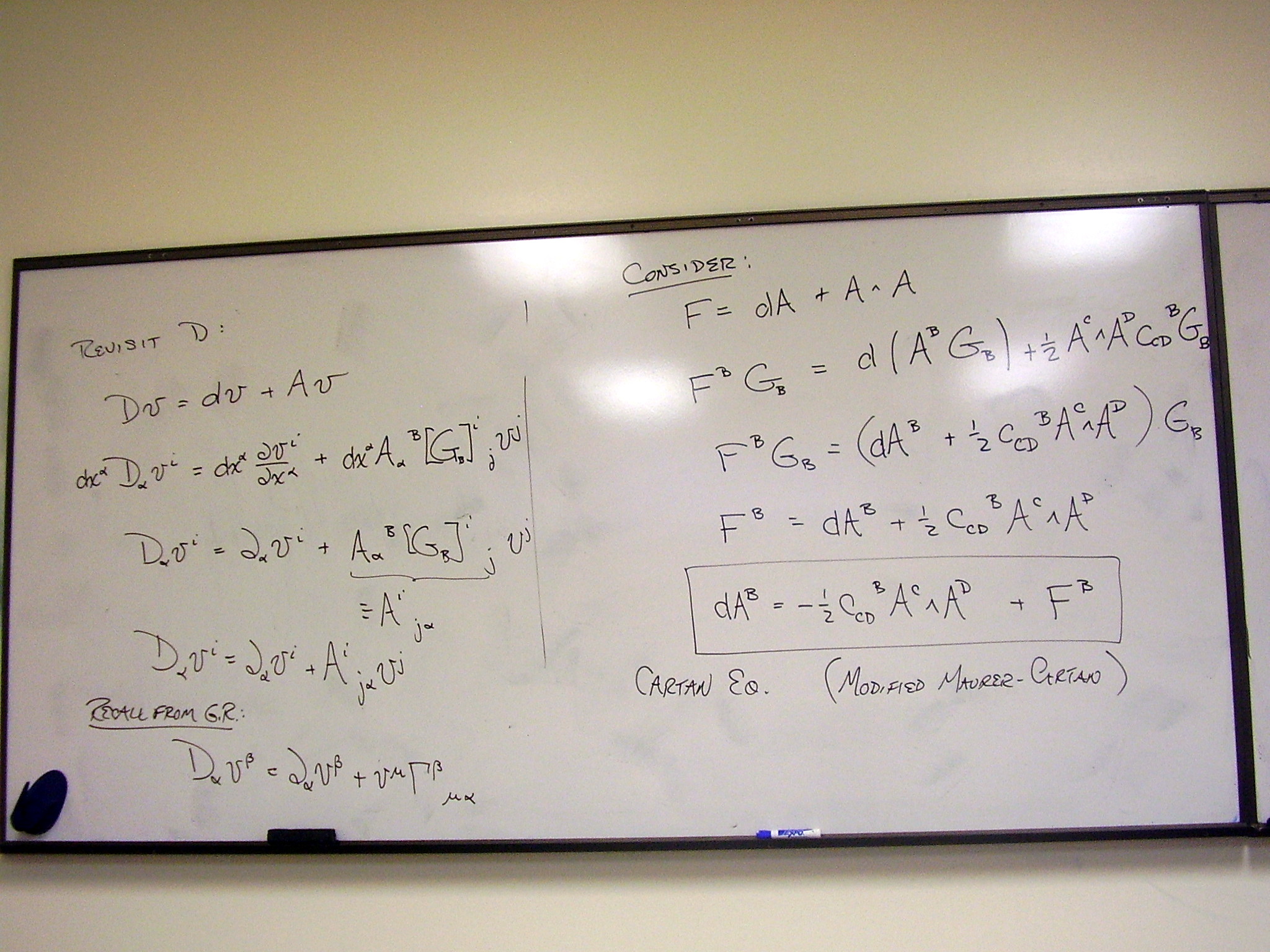
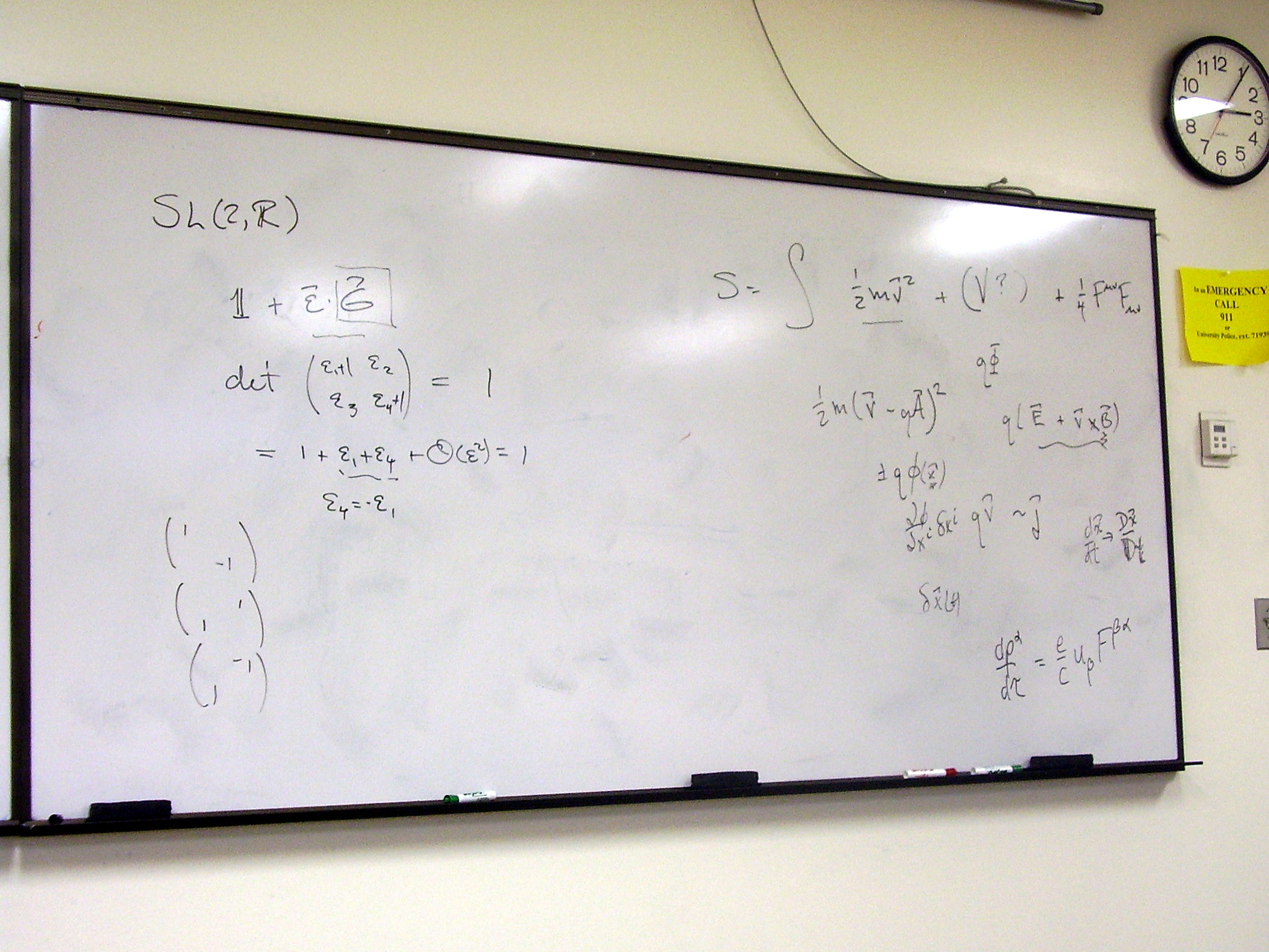
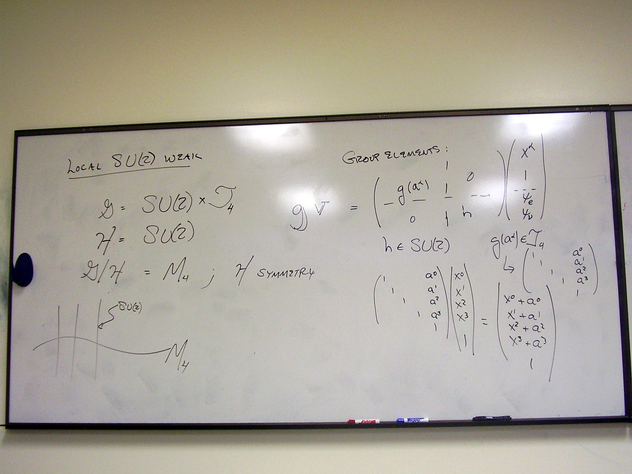
A simple gauge theory:
Electromagnetism as a U(1) x T4 gauge theory:
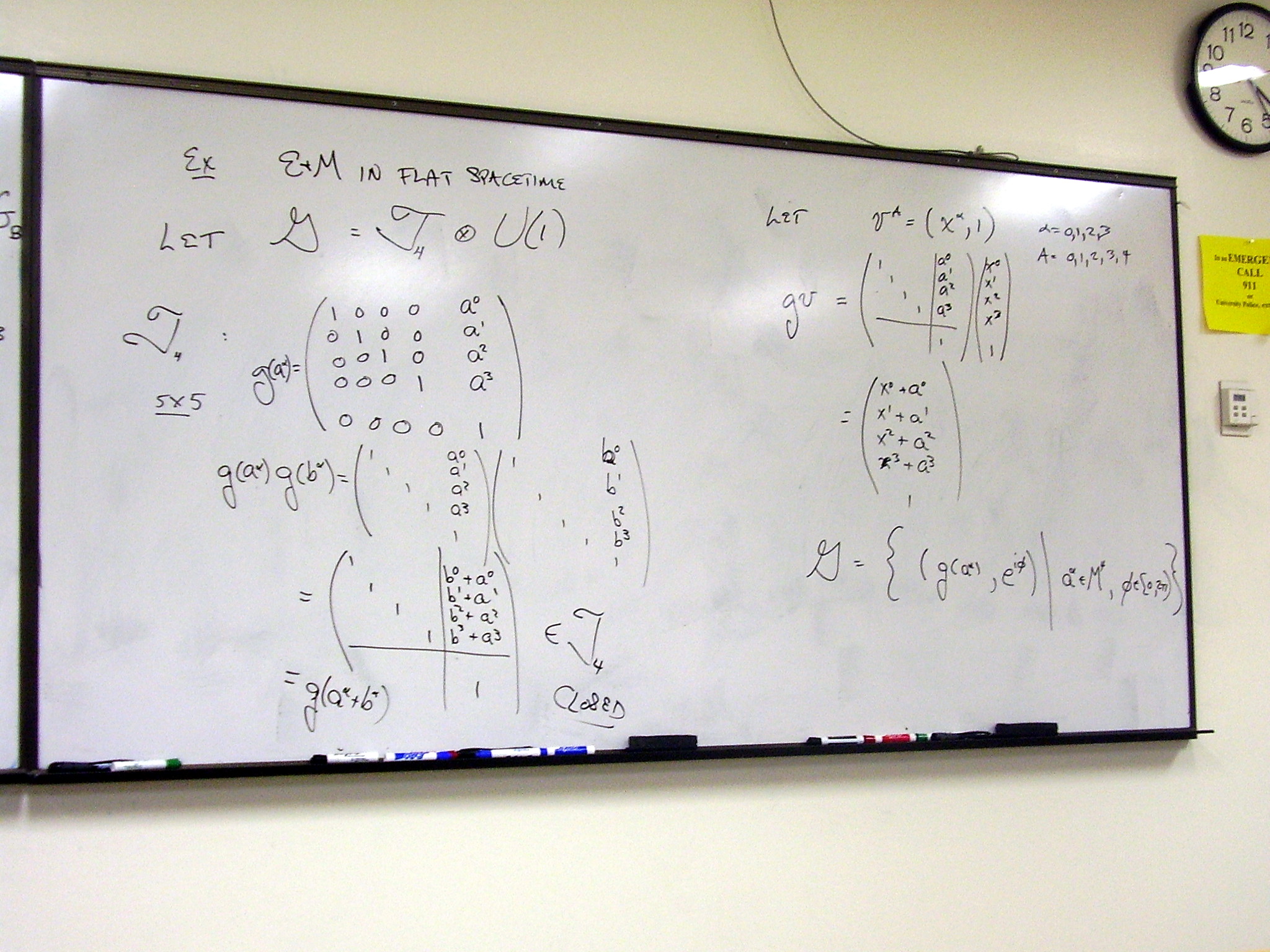
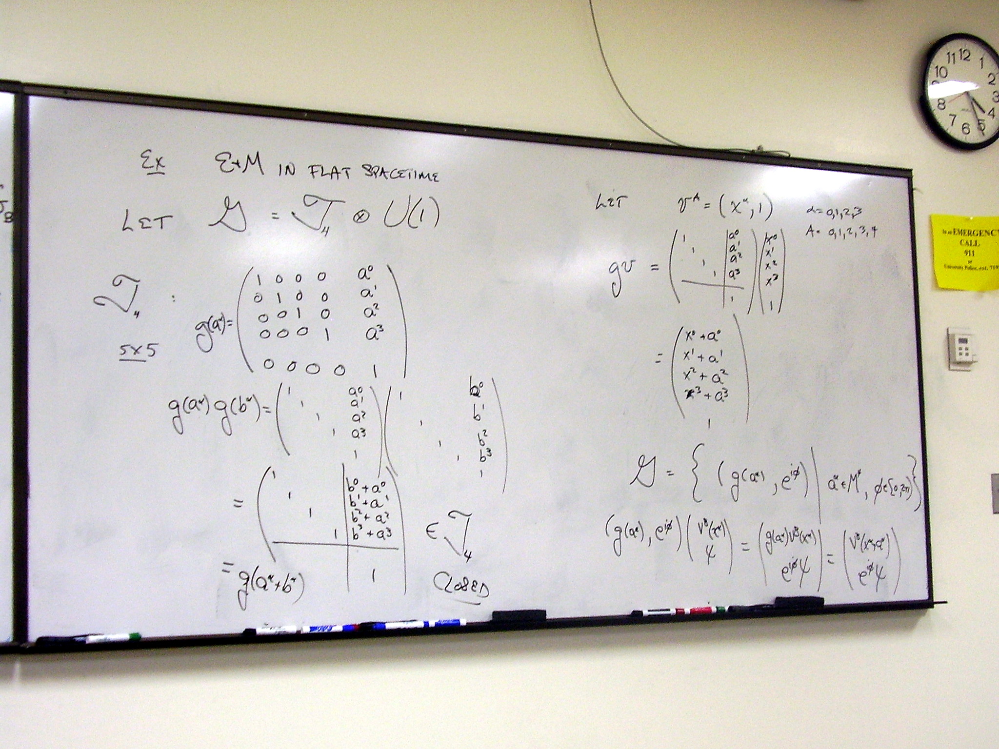
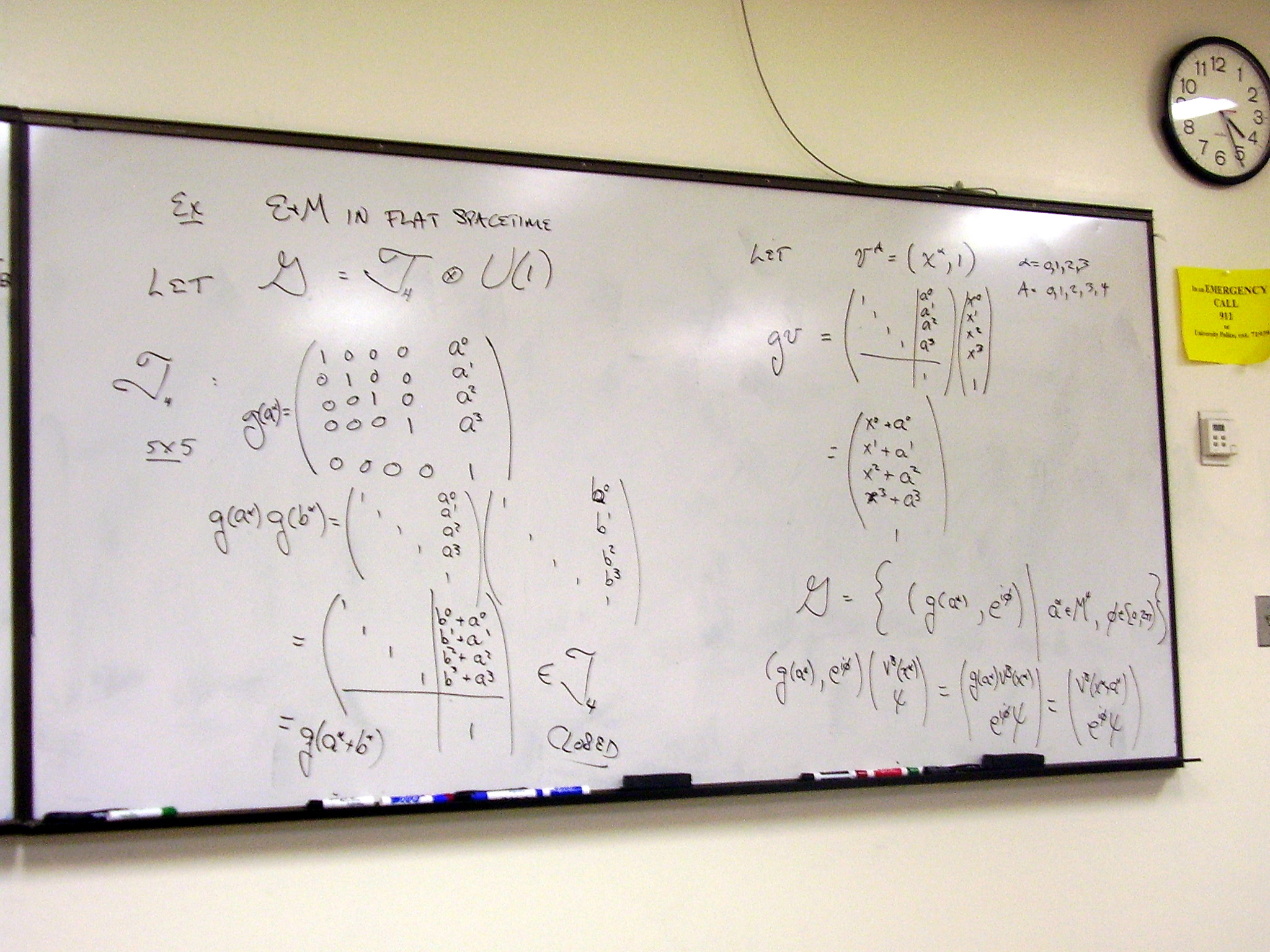
Wednesday, February
25, 2009
The exponential as the limit
of a product. Inductive proof of the binomial theorem:
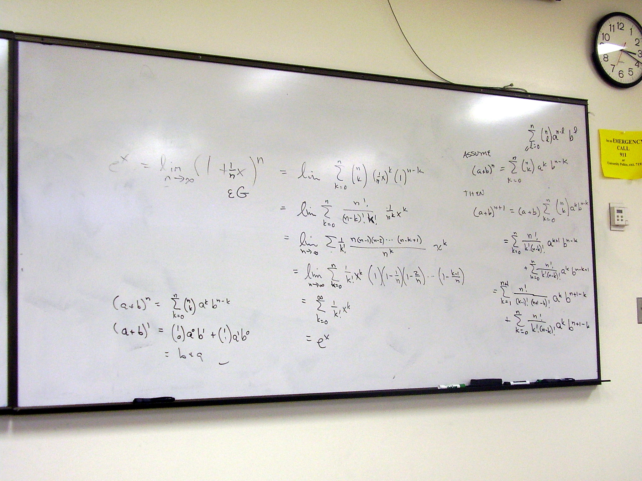
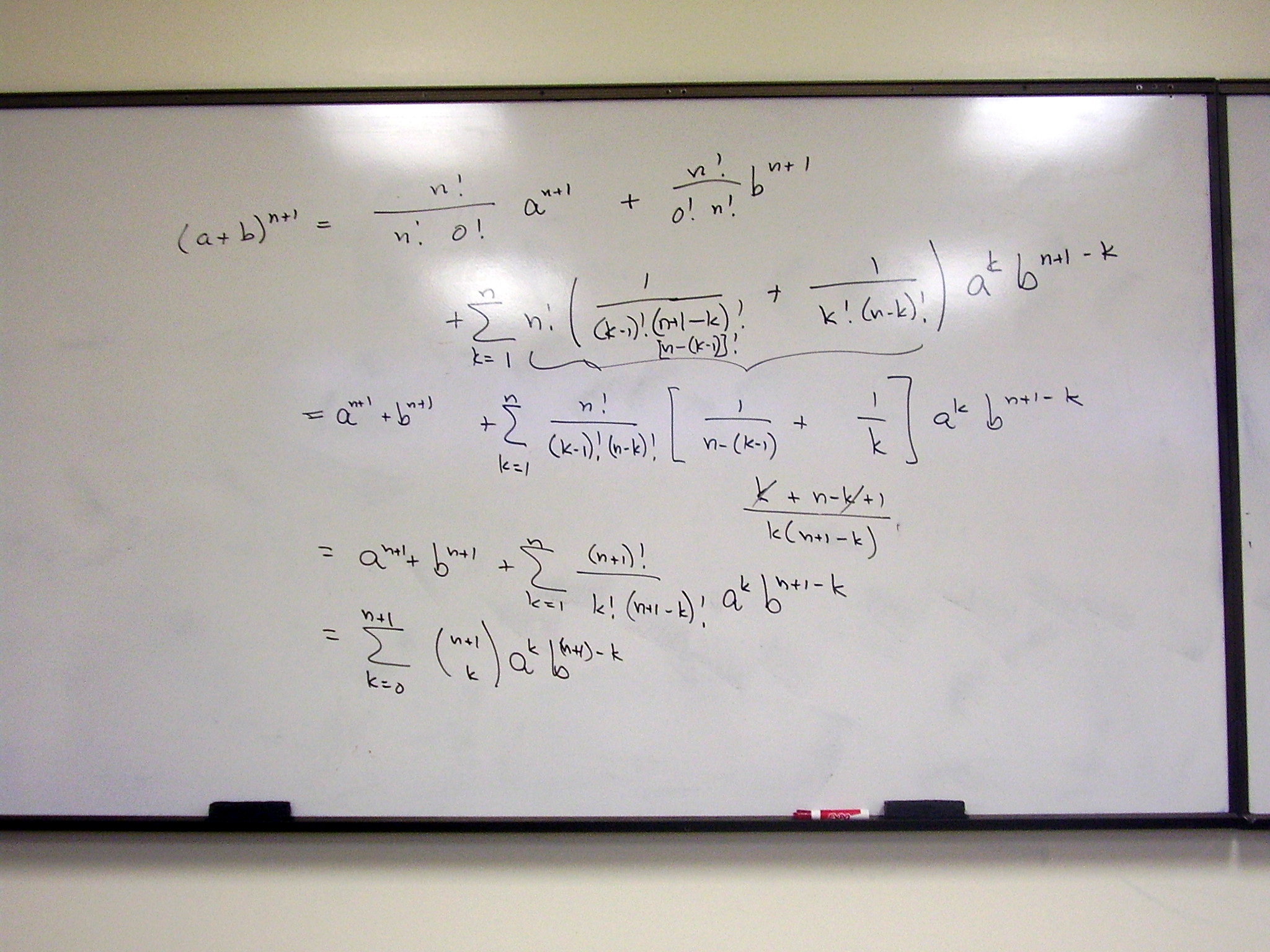
The exterior derivative of a
product:
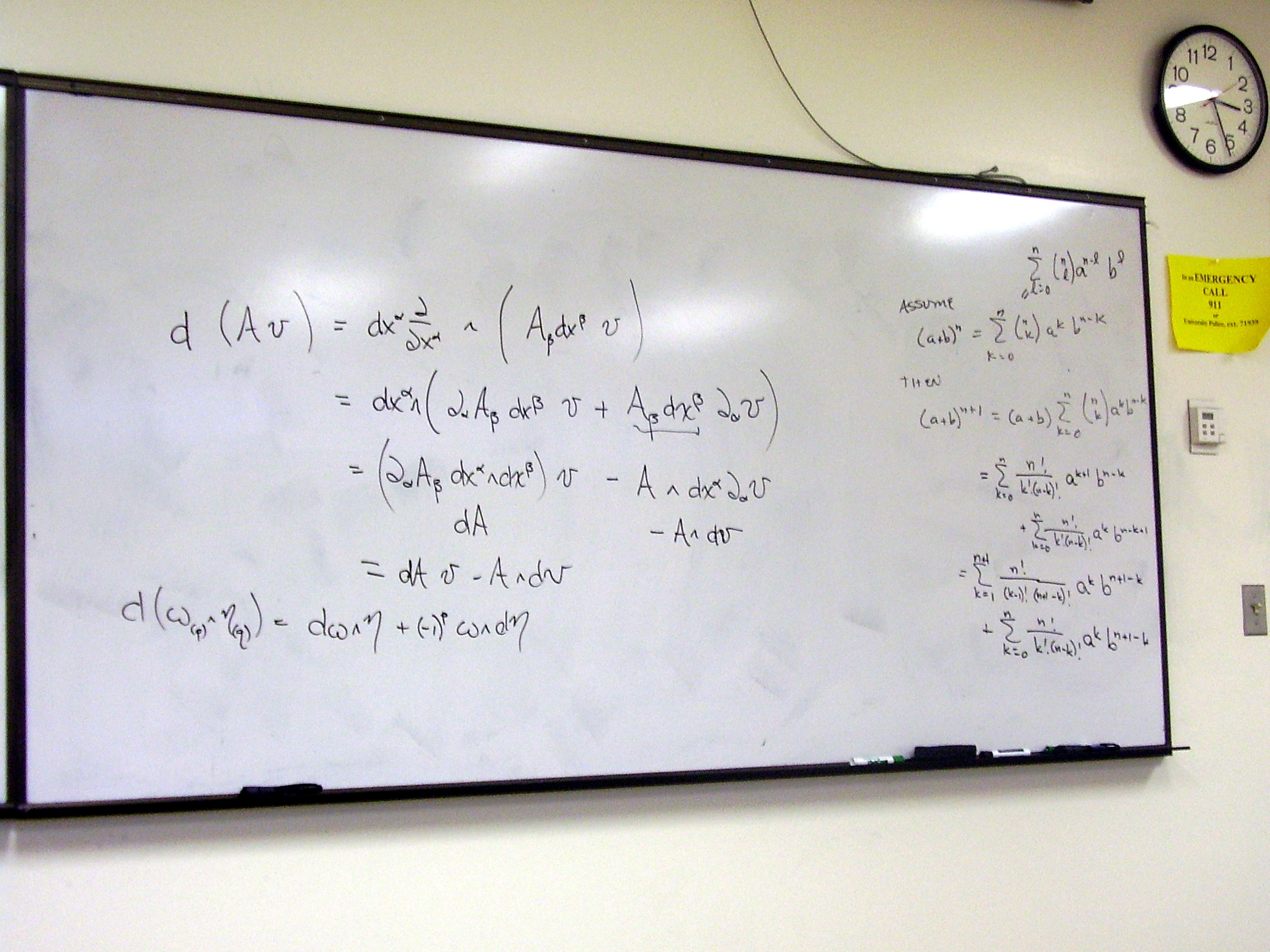
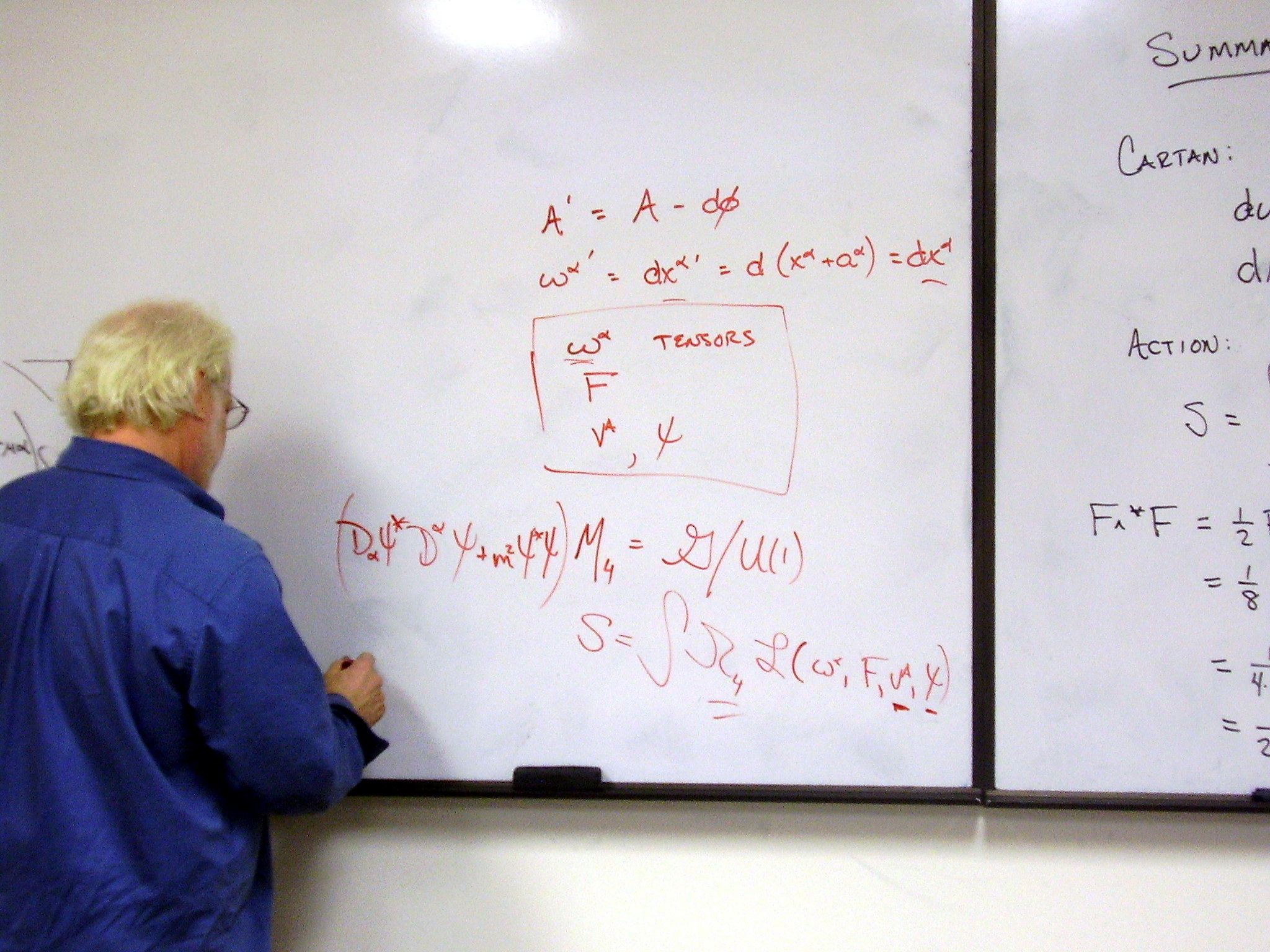
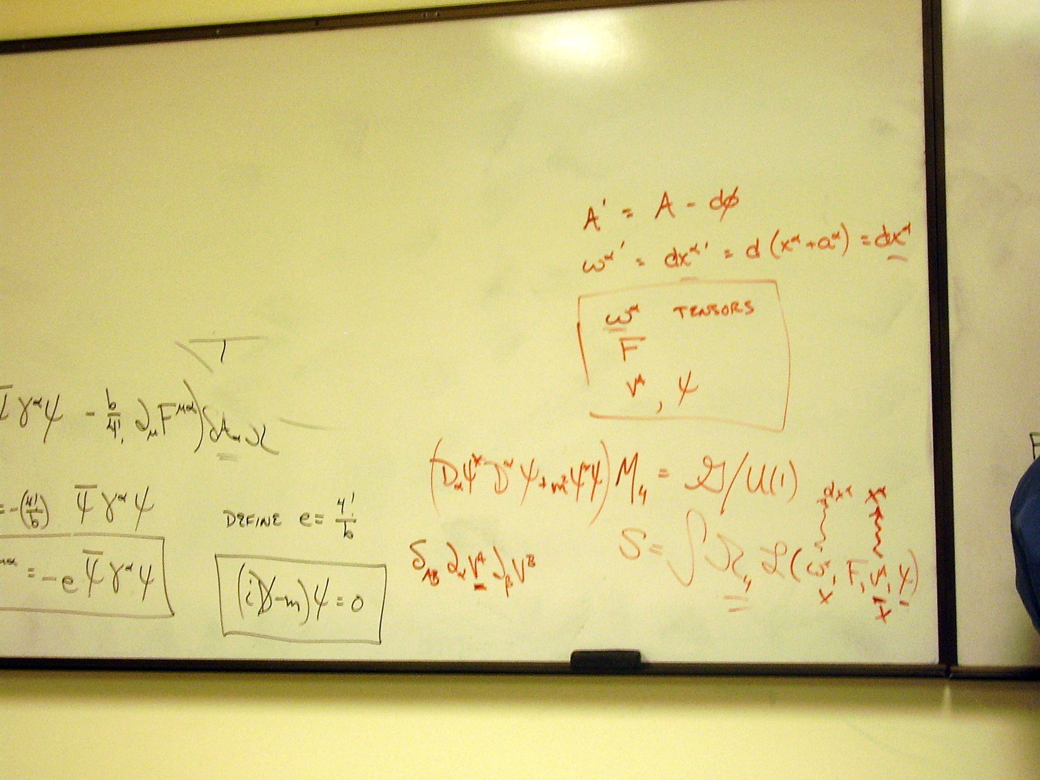
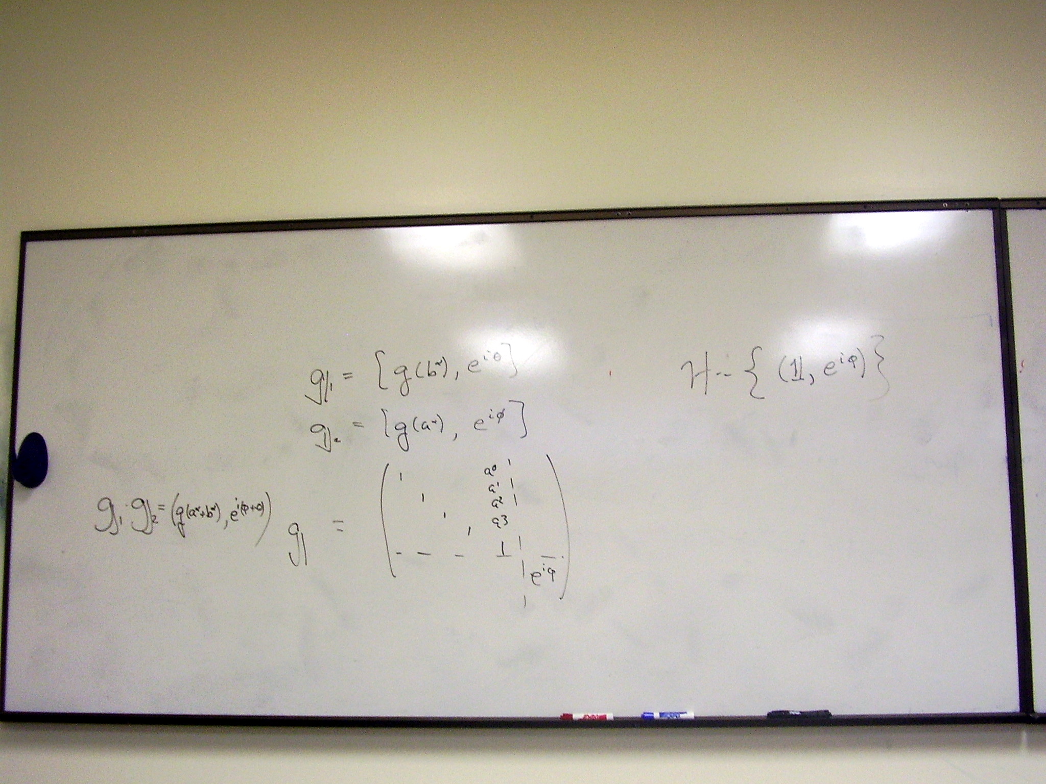
Gauging U(1). Define a
linear representation of T4 x U(1), where T4 is the group of four translations. Find
the infinitesimal generators:
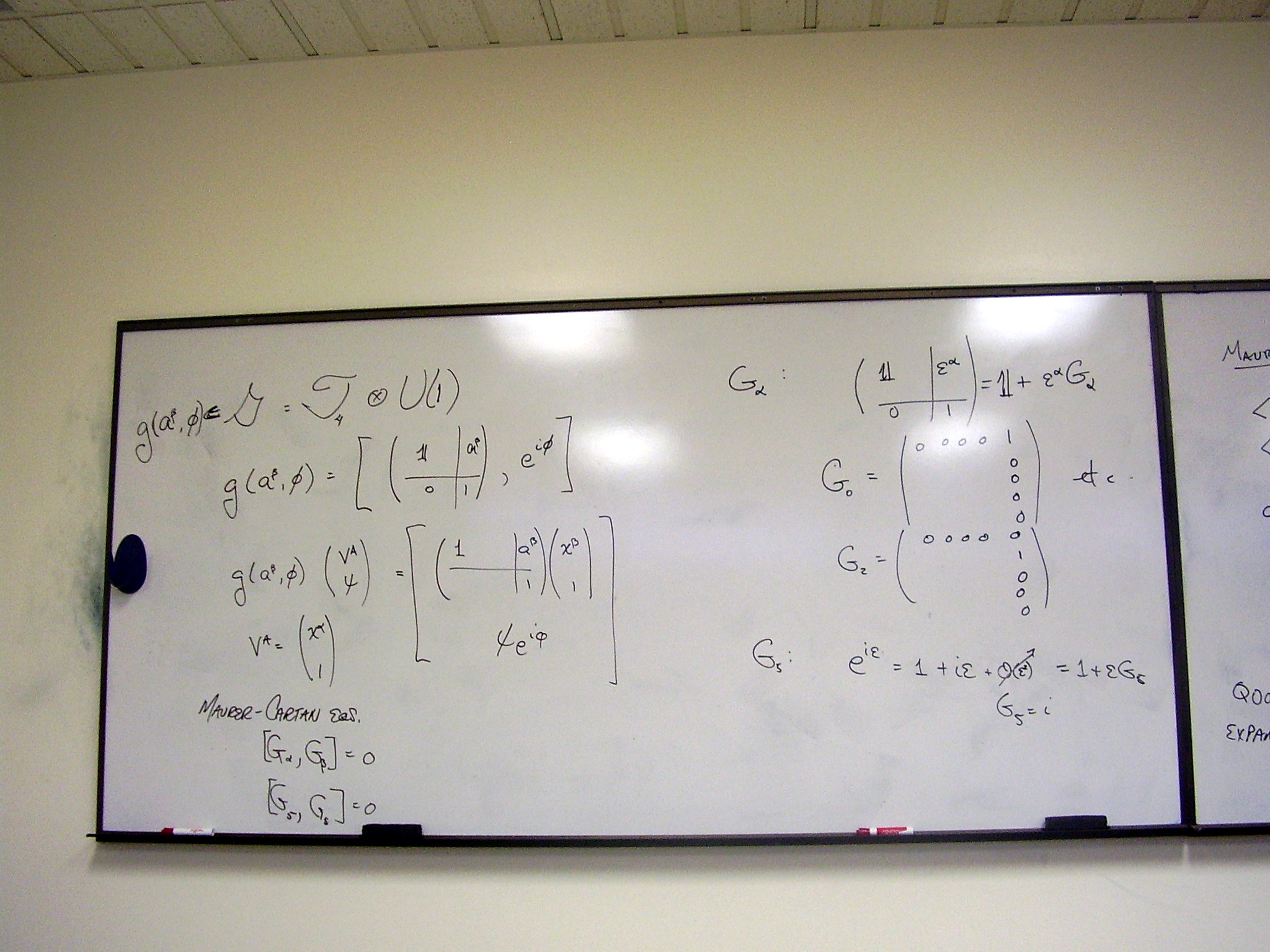
Define 1-forms dual to the
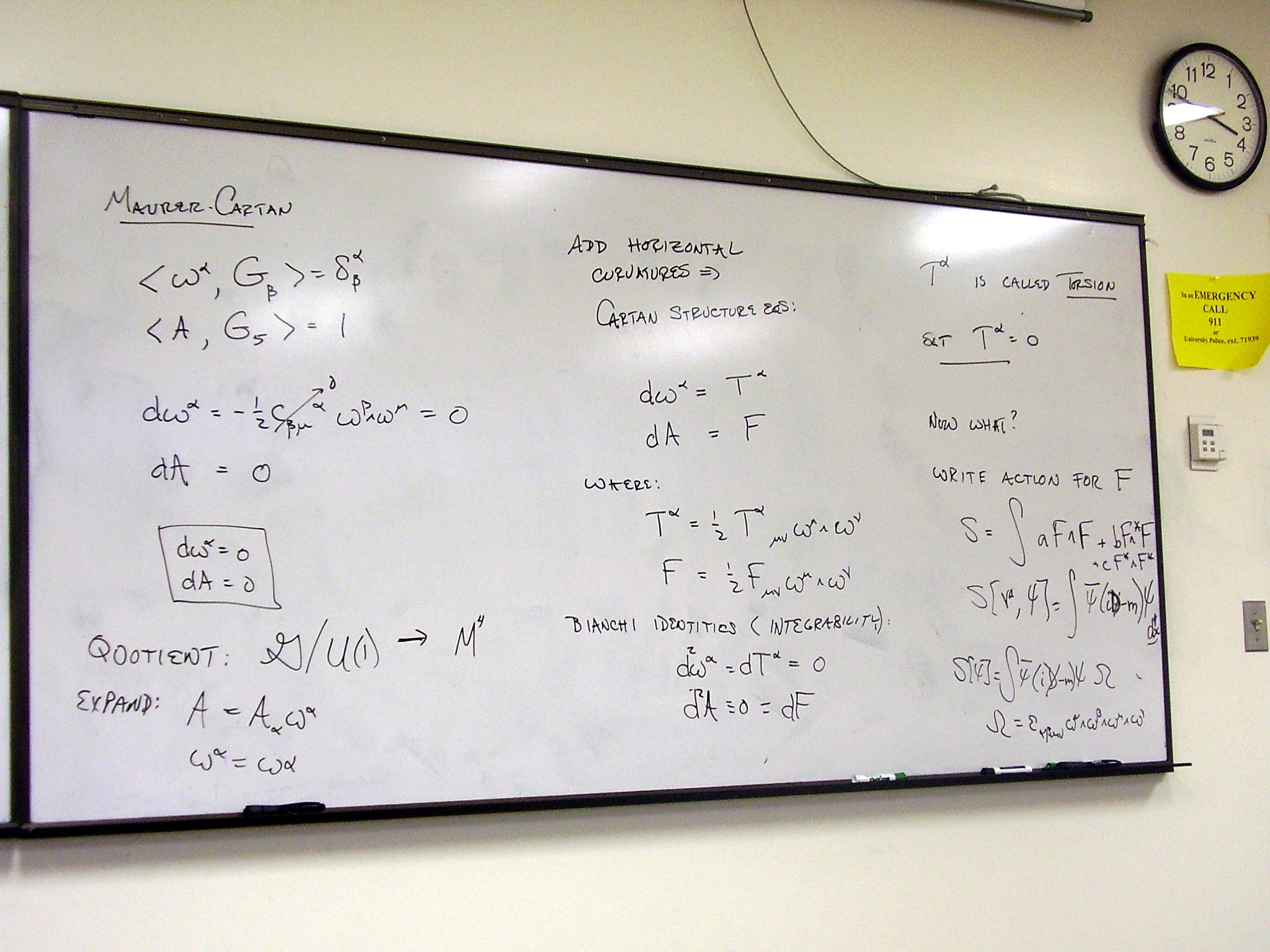
generators; write the Maurer-Cartan structure equations; take the quotient
[ T4 x U(1) ] / U(1)
to get a U(1) fiber bundle
over spacetime. Generalize the connection to introduce curvatures: a U(1)
curvature F and torsion for the translations. Write an action functional in
terms of the curvatures and any available tensors.
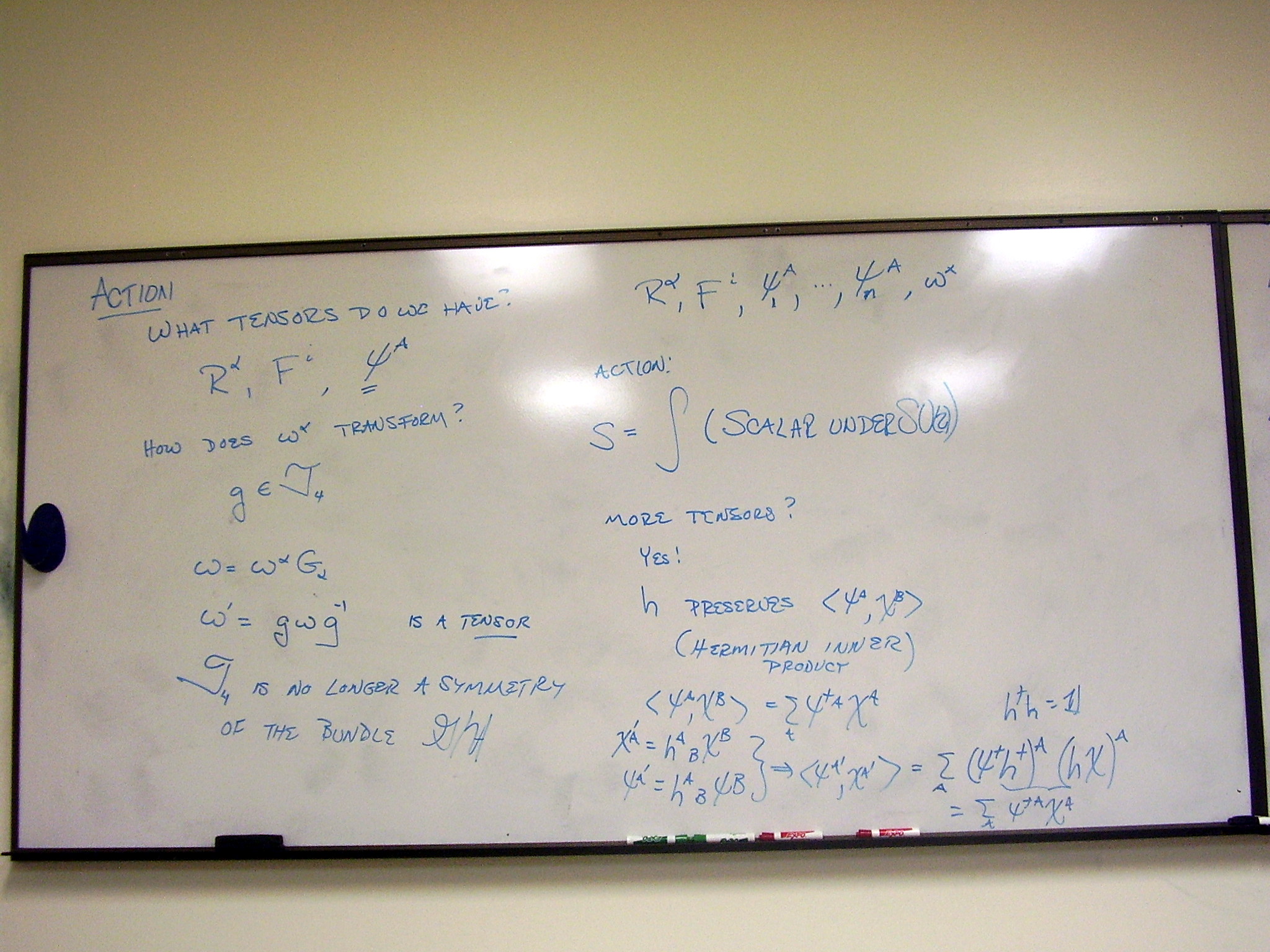
Expand possible curvature
terms:
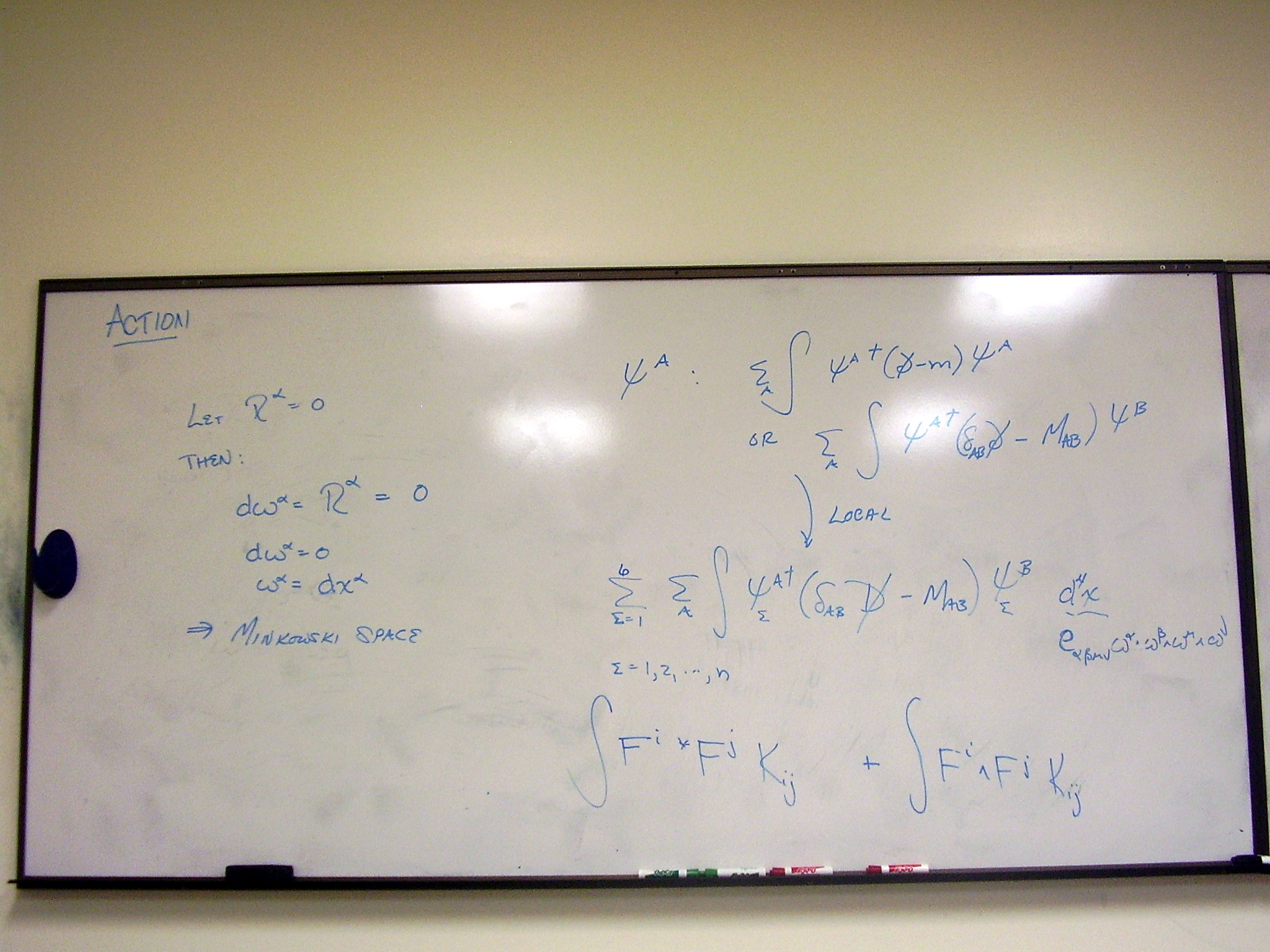
Write the most general
quadratic action; add matter terms. Vary the action to find the Dirac and
Maxwell equations:
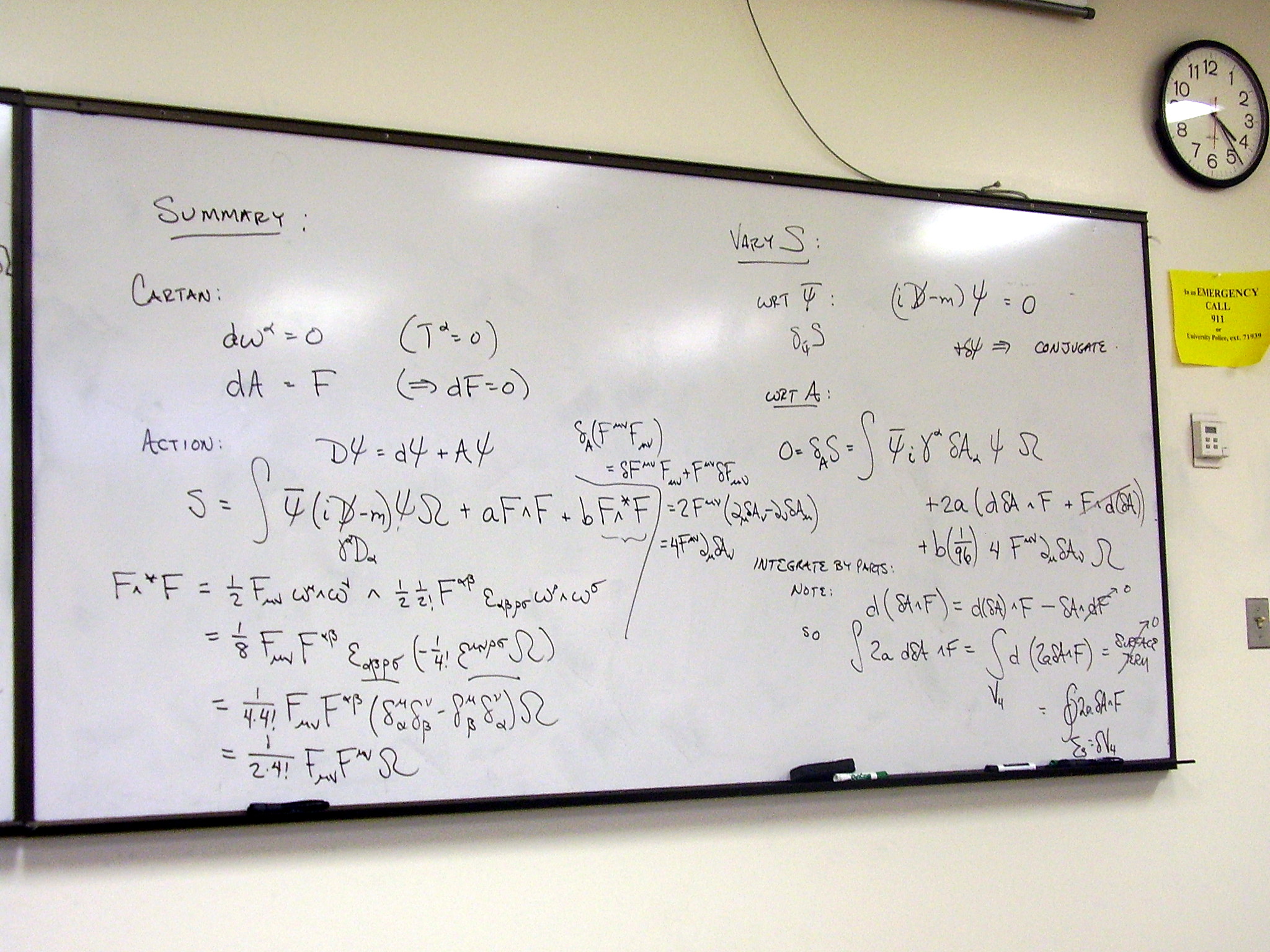
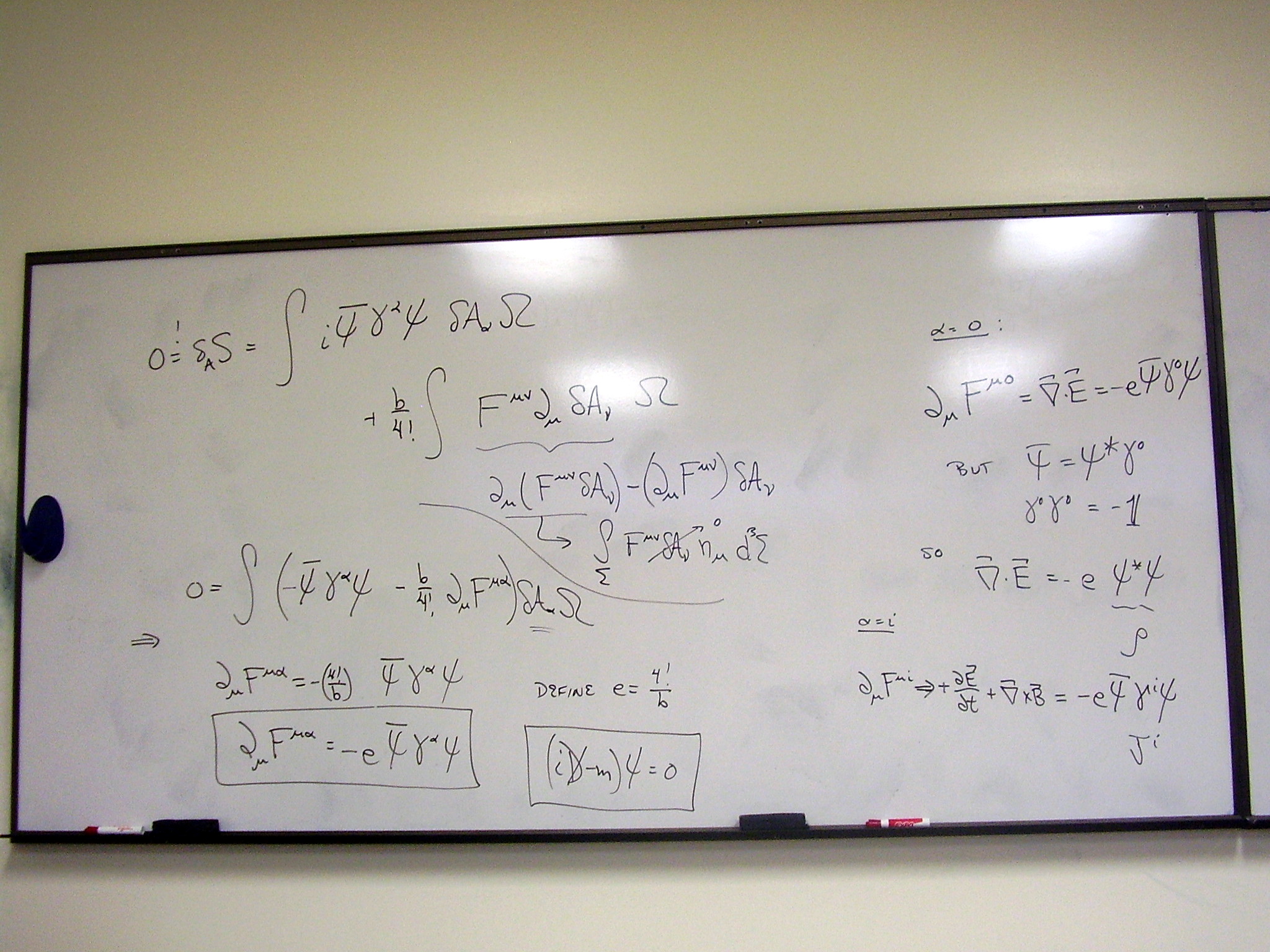
Available tensors:
Friday, February 27,
2009
The gauging procedure
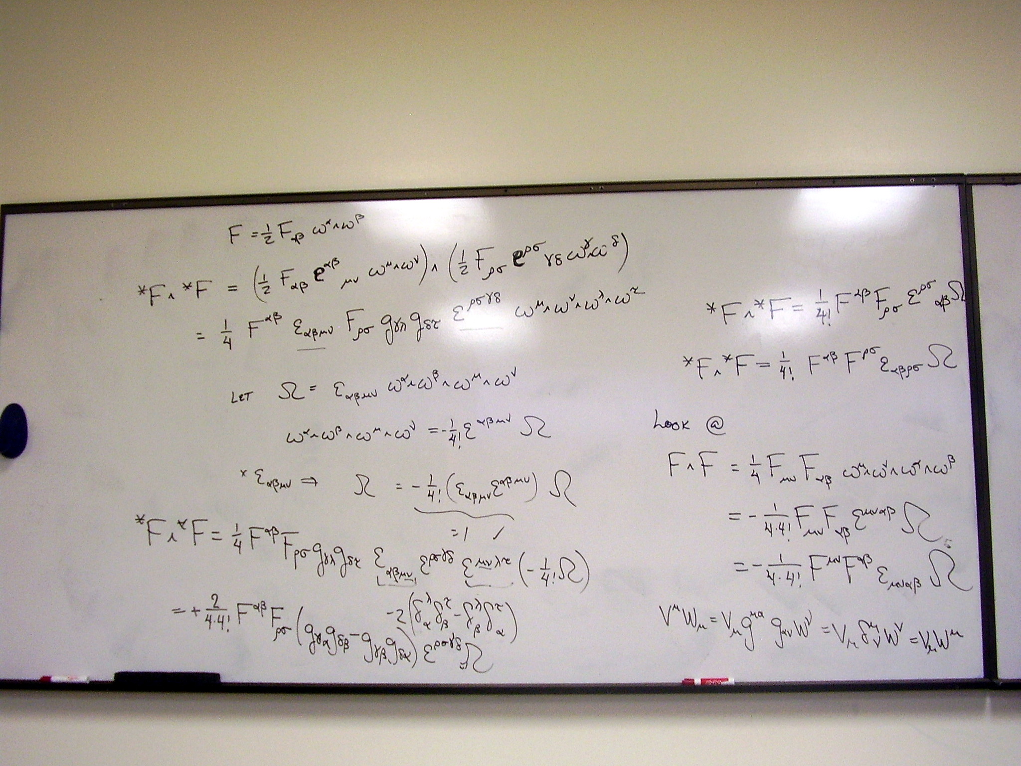
Various comments: U(1); Integrability conditions and the
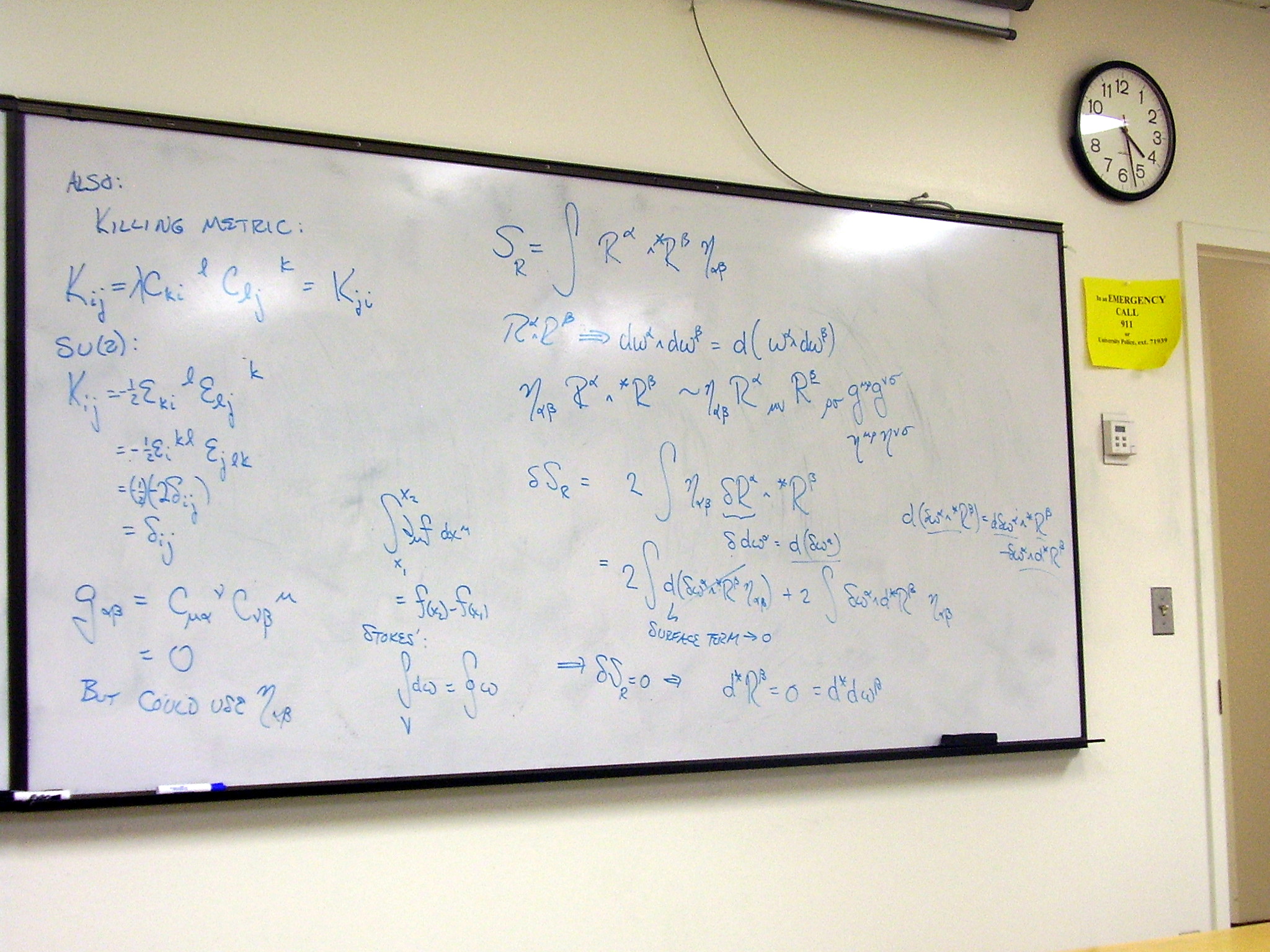
Bianchi identities; identity with the Levi-Civita tensor:
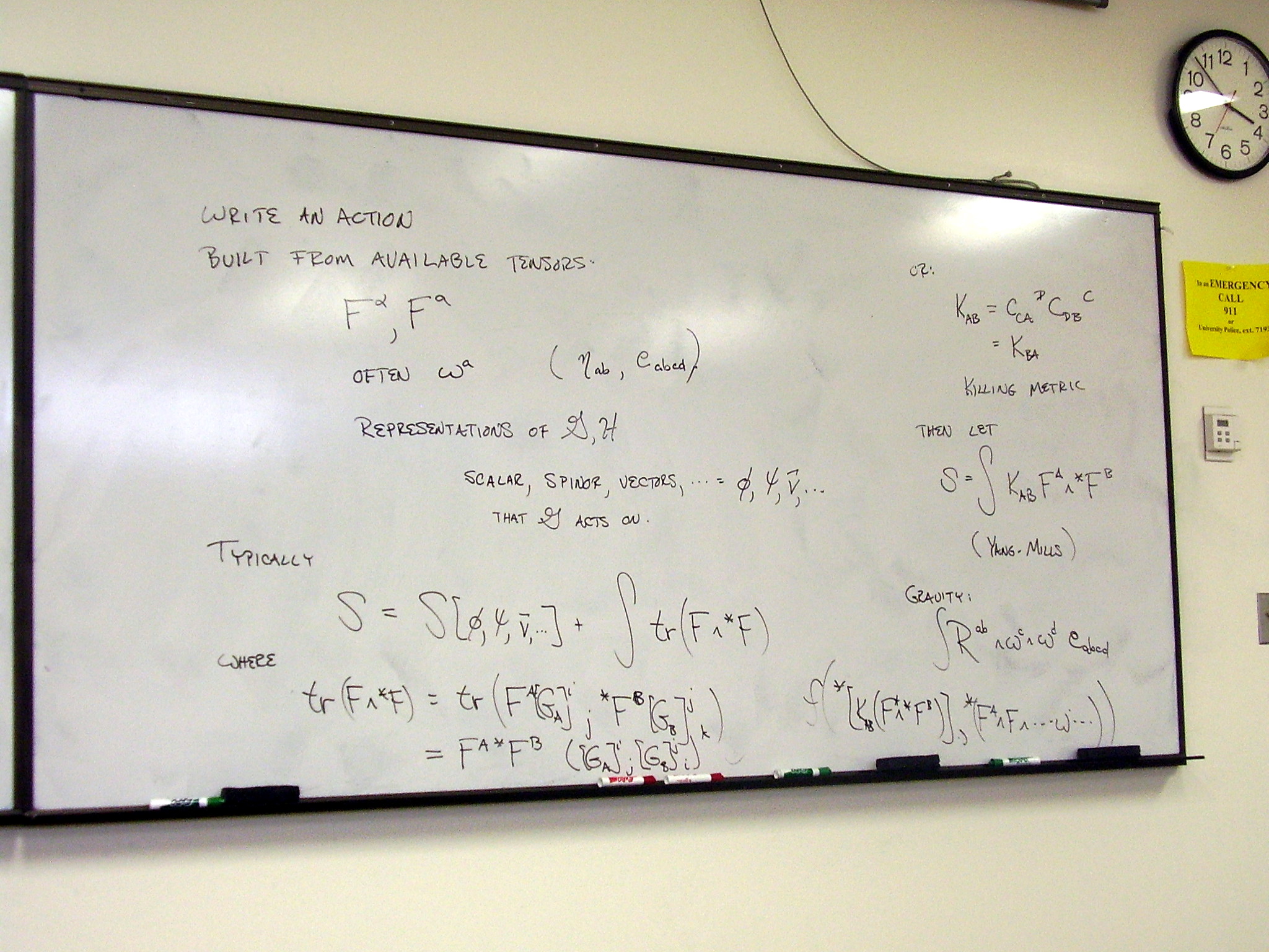
Summary of the gauging procedure:
1.
Identify a
relevant symmetry to make local; include a translation subgroup to provide a
base manifold.
2. Find
the structure constants of the Lie algebra and write the Maurer-Cartan
structure equations.
3. Take
the quotient of the group by the desired local symmetry subgroup.
4. Cartan
structure eqs.: Generalize the connection, leading to the addition of
horizontal curvature 2-forms.
5. Identify
tensors by studying the gauge transformations of the connection and curvature.
6. Build
an invariant action (usually) from the available tensors.
7. Vary
the action with respect to all connection 1-forms to find the field equations.
8. Solve
the combined system of field equations and Cartan equations for the connection
and curvatures.
Monday, March 2, 2009
Linear representation of
U(1) x T4
Miscellaneous comments
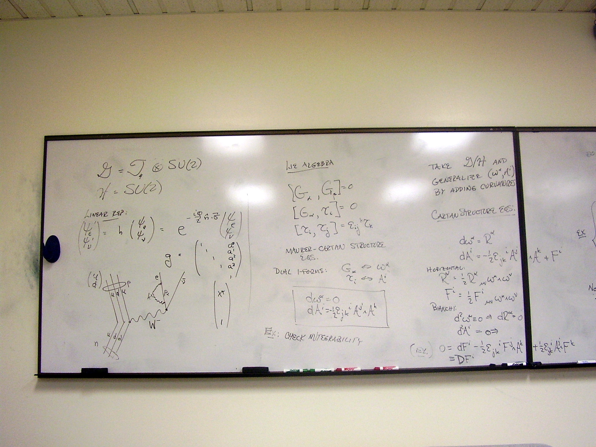
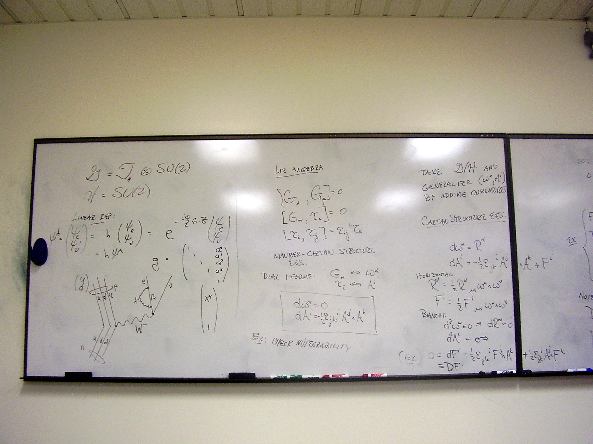
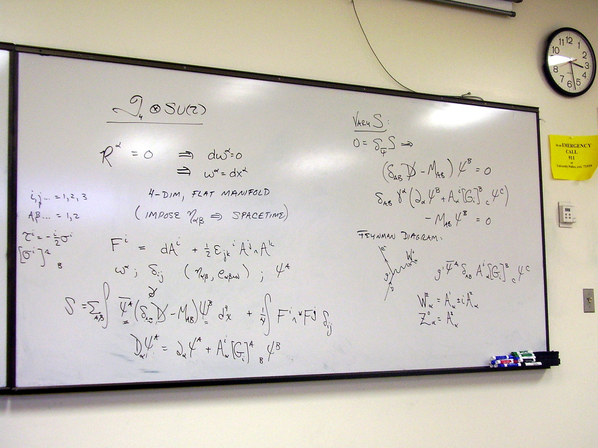
SU(2) gauge theory:
Dirac action for two
fermions with global SU(2) symmetry:
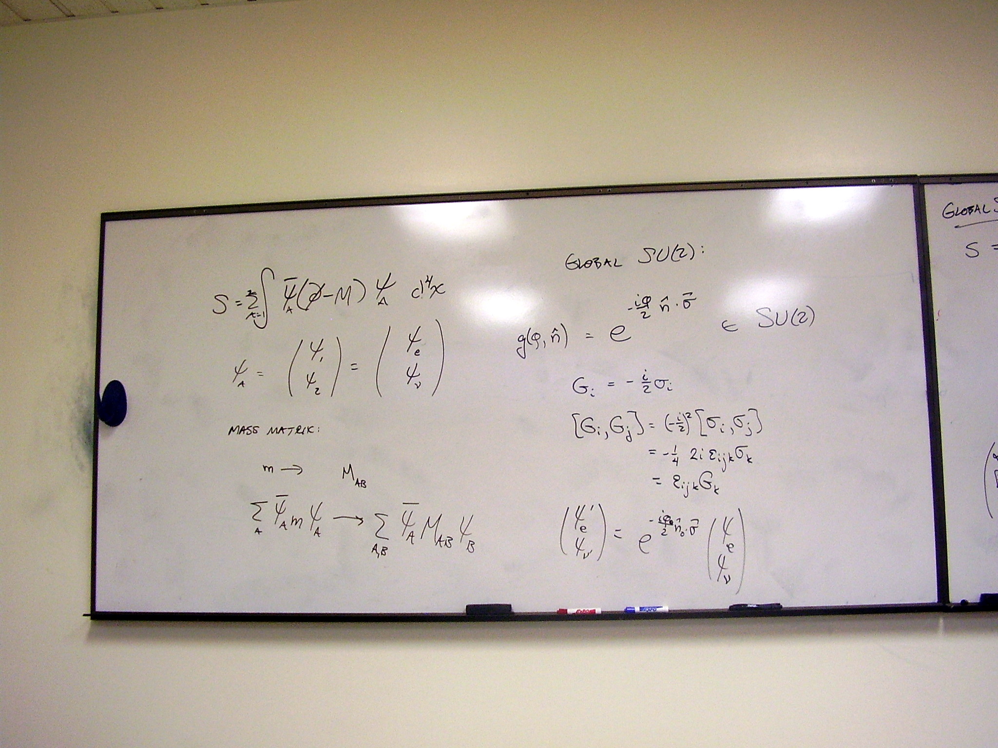
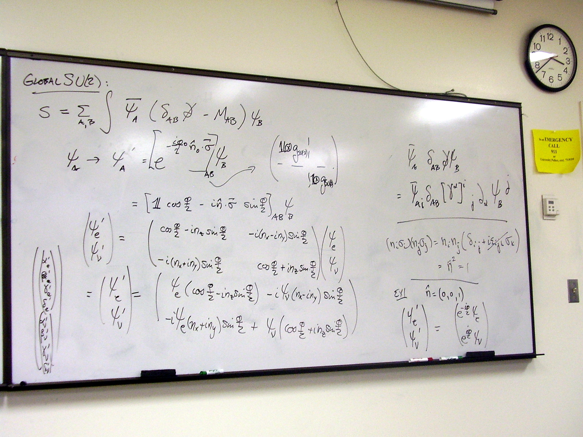
Gauging to local SU(2)
symmetry on spacetime: Linear representation of SU(2) x T4; the Lie
algebra; Cartan structure equations; action:
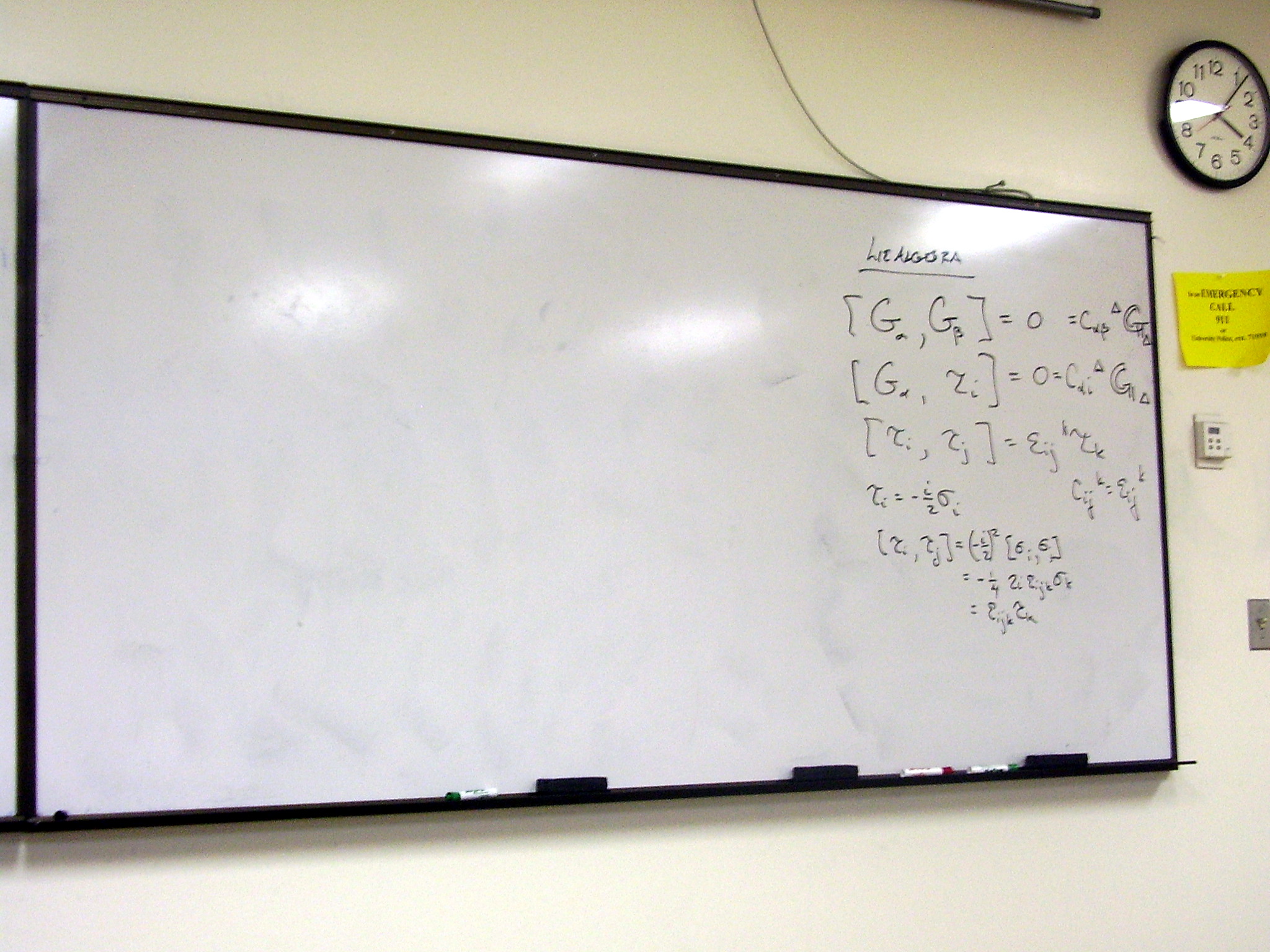
Wednesday, March 4,
2009
Lecture:
SU(2) gauge theory, continued
Question on generalized
Stokes’ theorem
Developing the Cartan
equations for SU(2) x T4 gauge theory:
Bianchi identity for the
SU(2) curvature. Exercises.
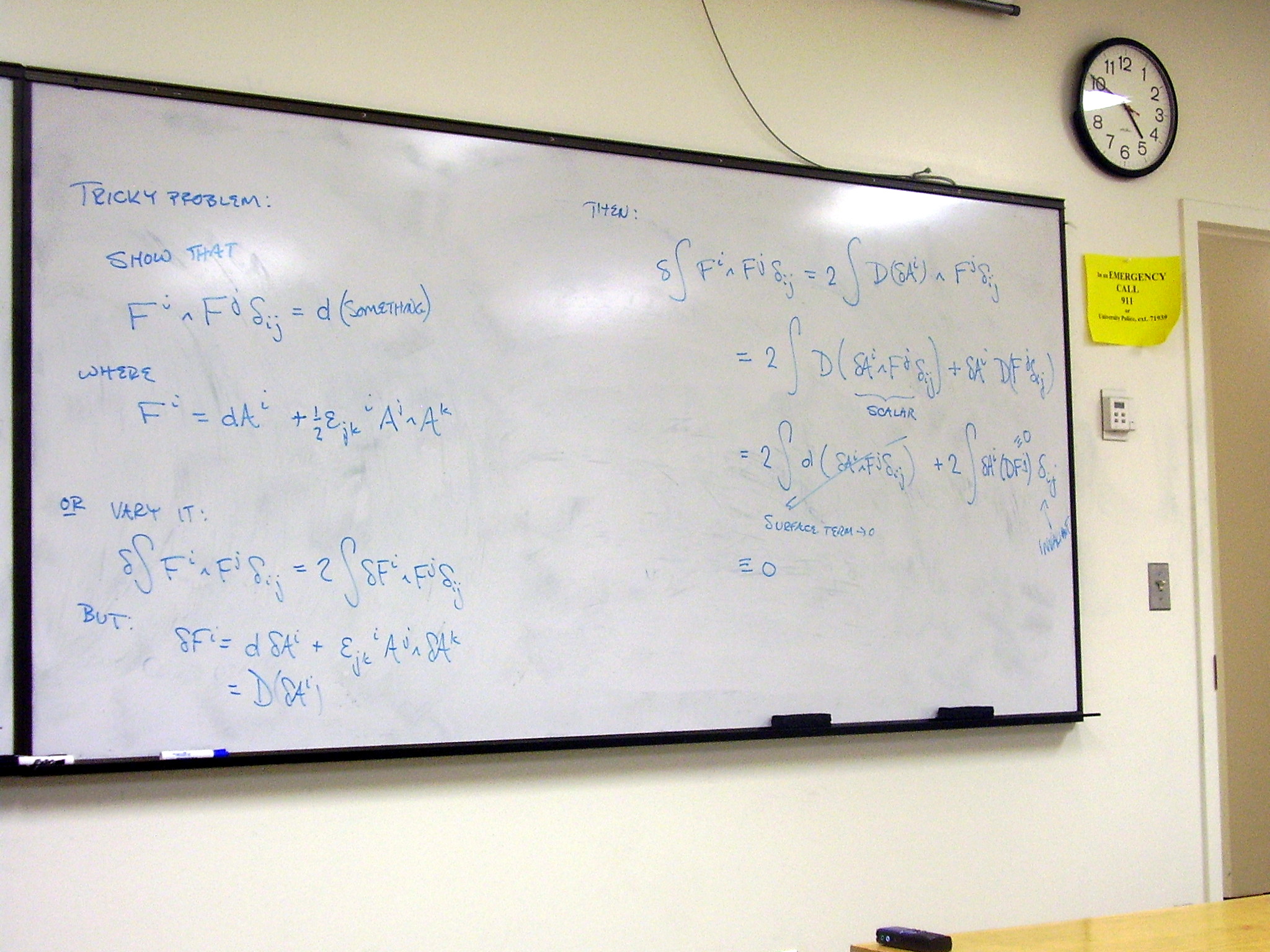
Torsion: the curvature of
local translations
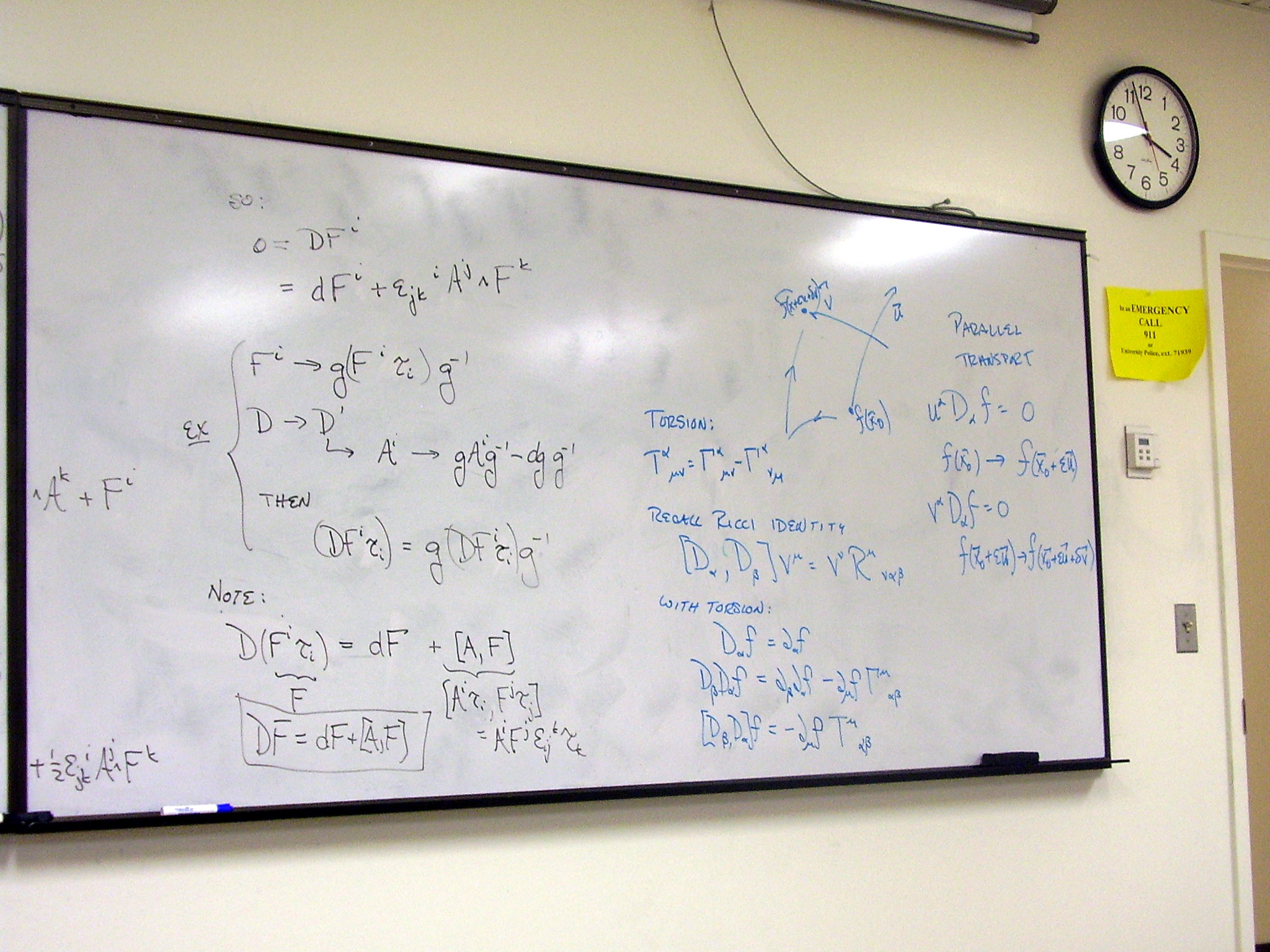
Writing an SU(2) invariant
action. Finding available SU(2) tensors. Action terms for torsion, SU(2) field
strength, spinors.
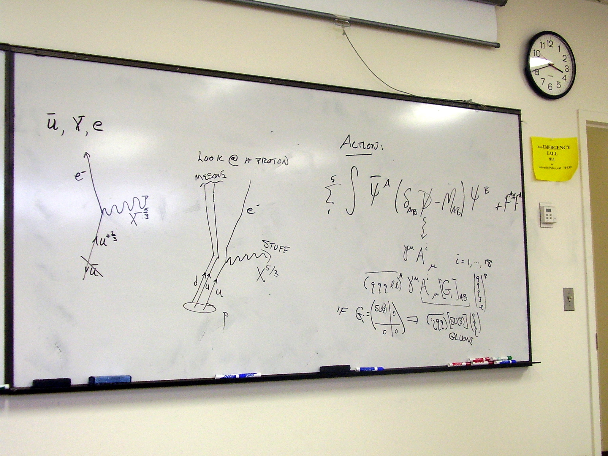
Friday, March 6, 2009
Interpreting SU(2) gauge theory: the
weak interaction
Recognizing subgroups from
the Lie algebra or Maurer-Cartan structure equations. Picturing the SU(2) fiber
bundle.
Interpreting the SU(2)
gauge theory. Varying the action. Spacetime and weak interactions.
The interaction term.
Feynman diagrams: picturing the weak interaction
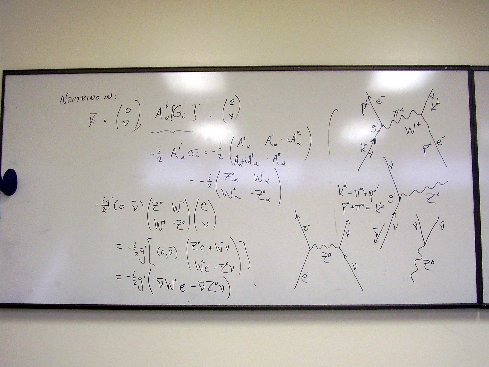
Varying the action with
respect to the gauge potentials: the Yang-Mills field equation
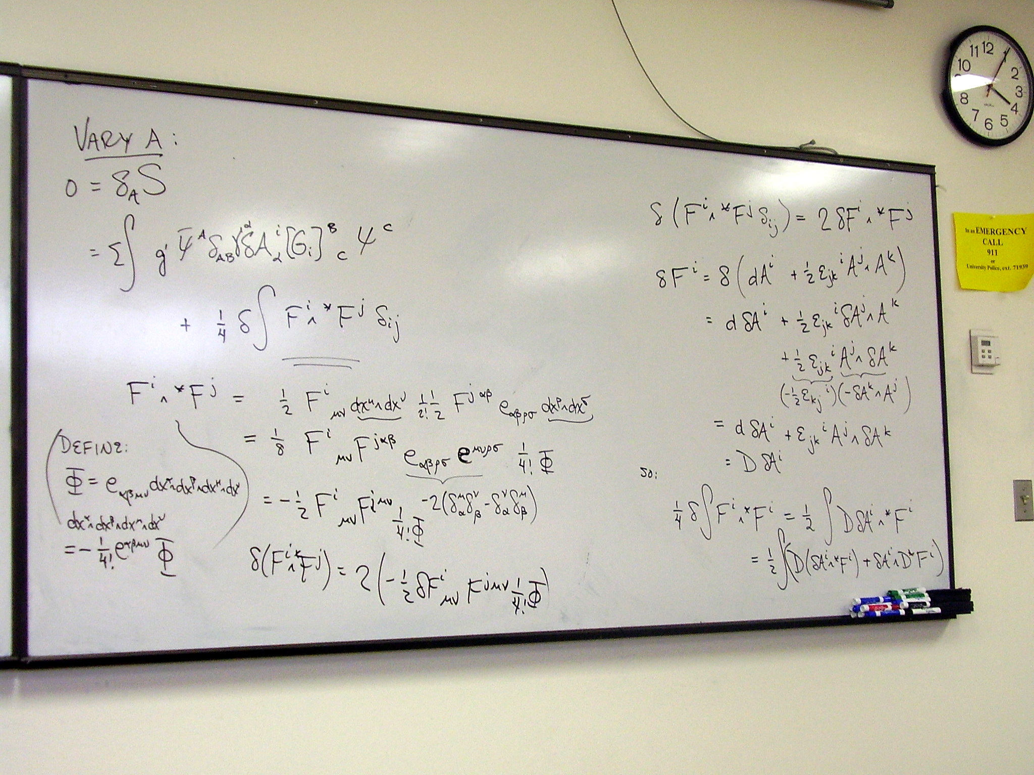
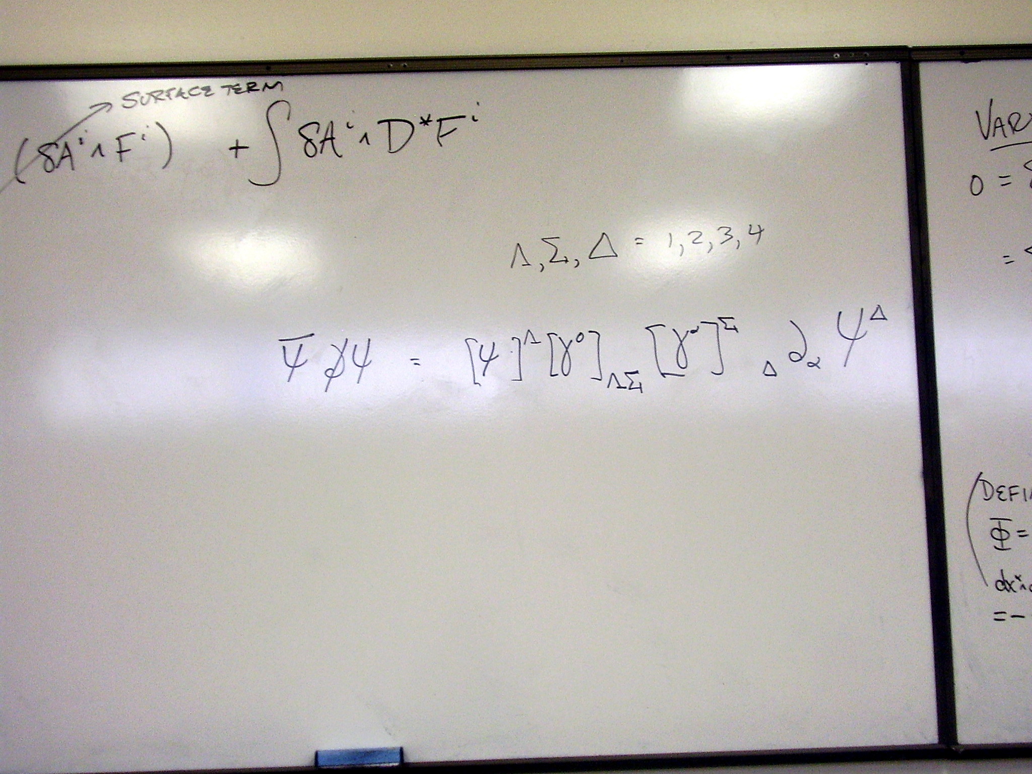
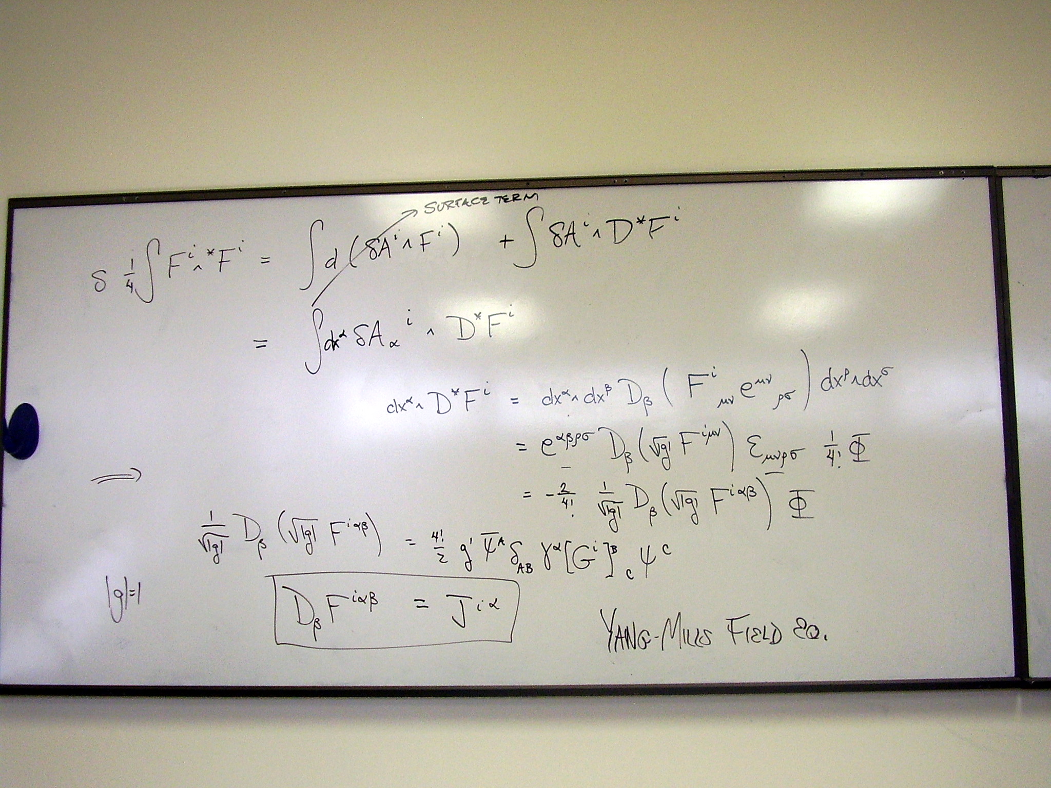
Interactions of the weak
intermediate vector bosons, with diagrams.
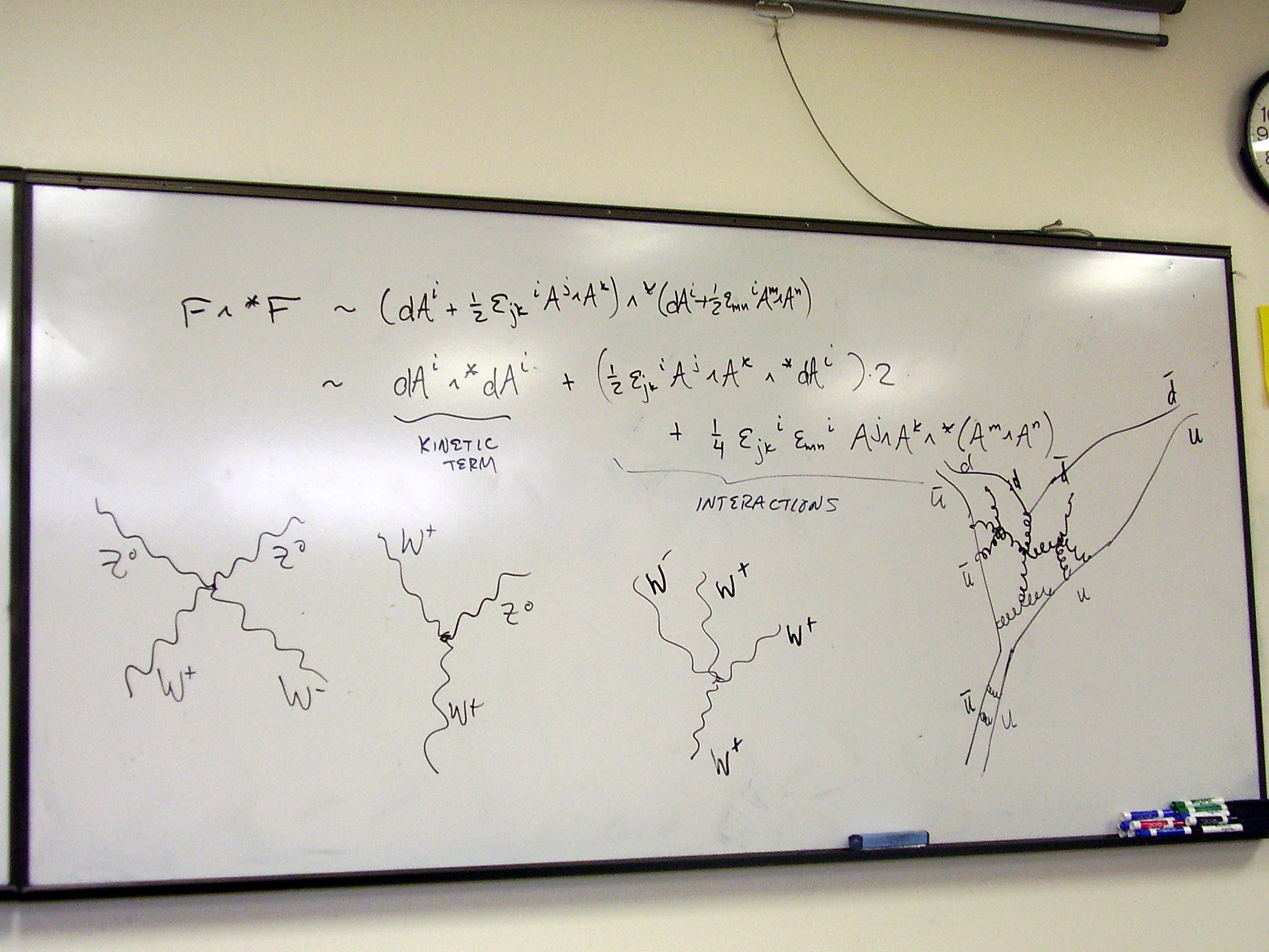
Monday, March 16, 2009
Conserved U(1) current for Dirac
particles
Conserved U(1) current for
the Dirac equation
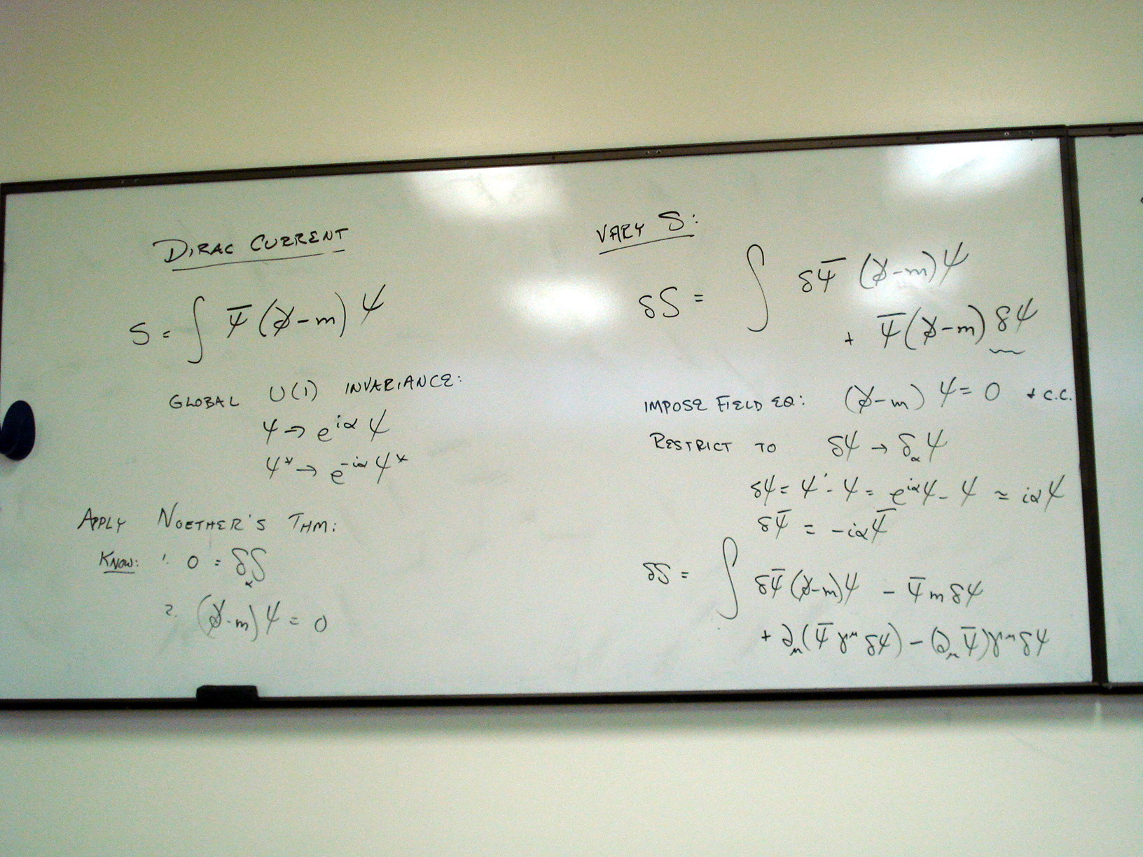
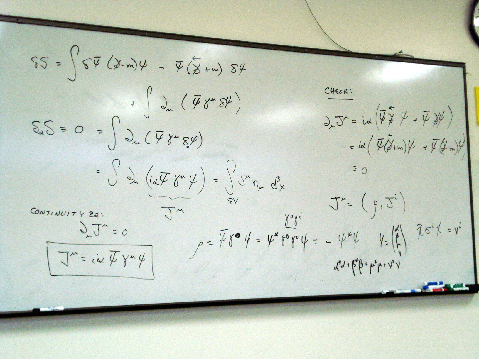
Explicit form in terms of
spinor components
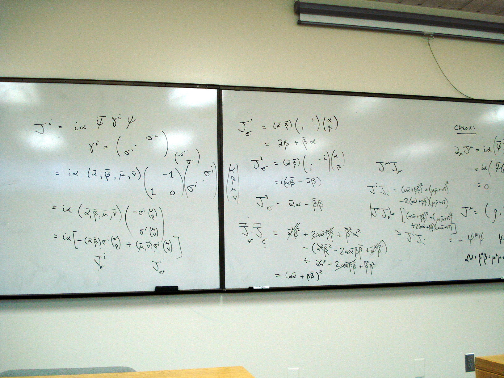
Feynman diagrams of three
fundamental interactions
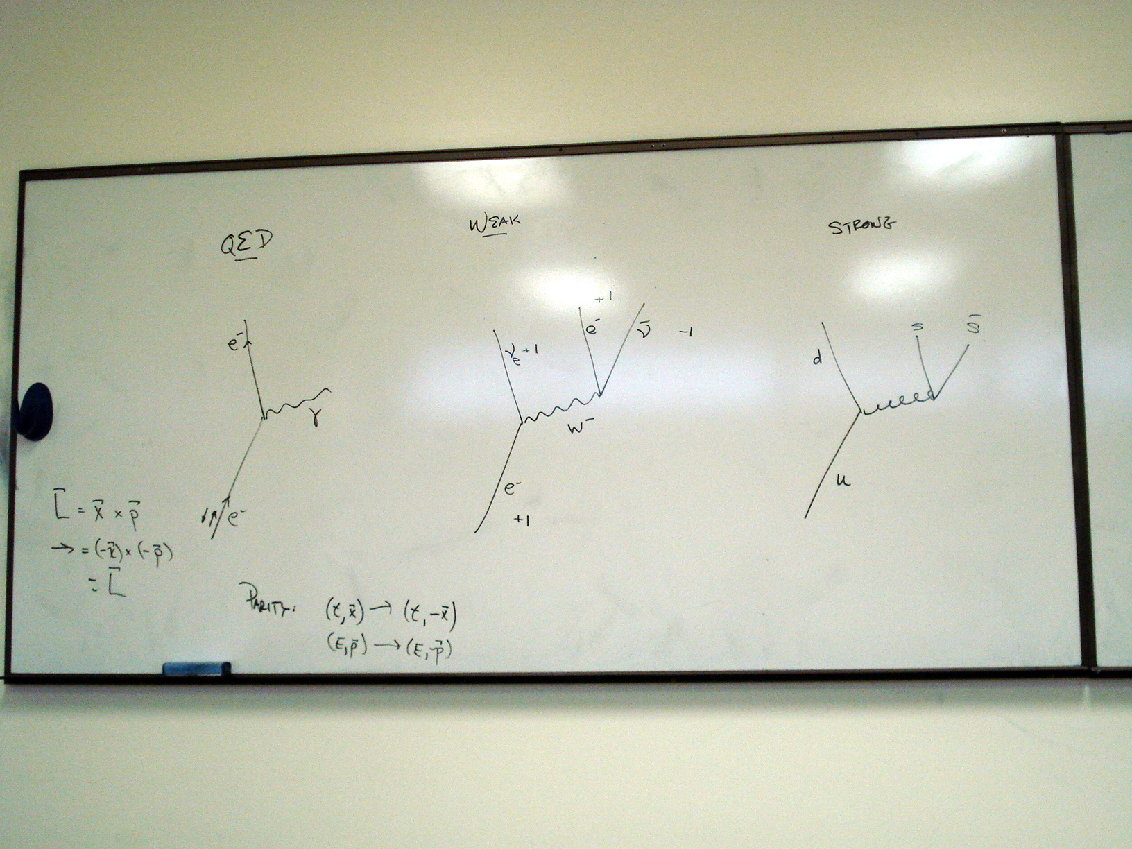
A possible decay
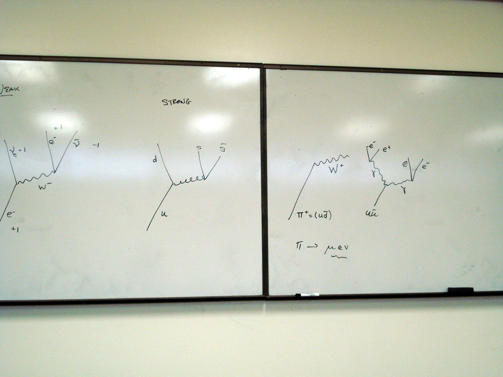
Wednesday, March 18,
2009
The Higgs mechanism. SU(5) grand
unified theory (GUT)
Electroweak mixing between
U(1) and the diagonal generator of SU(2) to give the photon and Z0
fields.
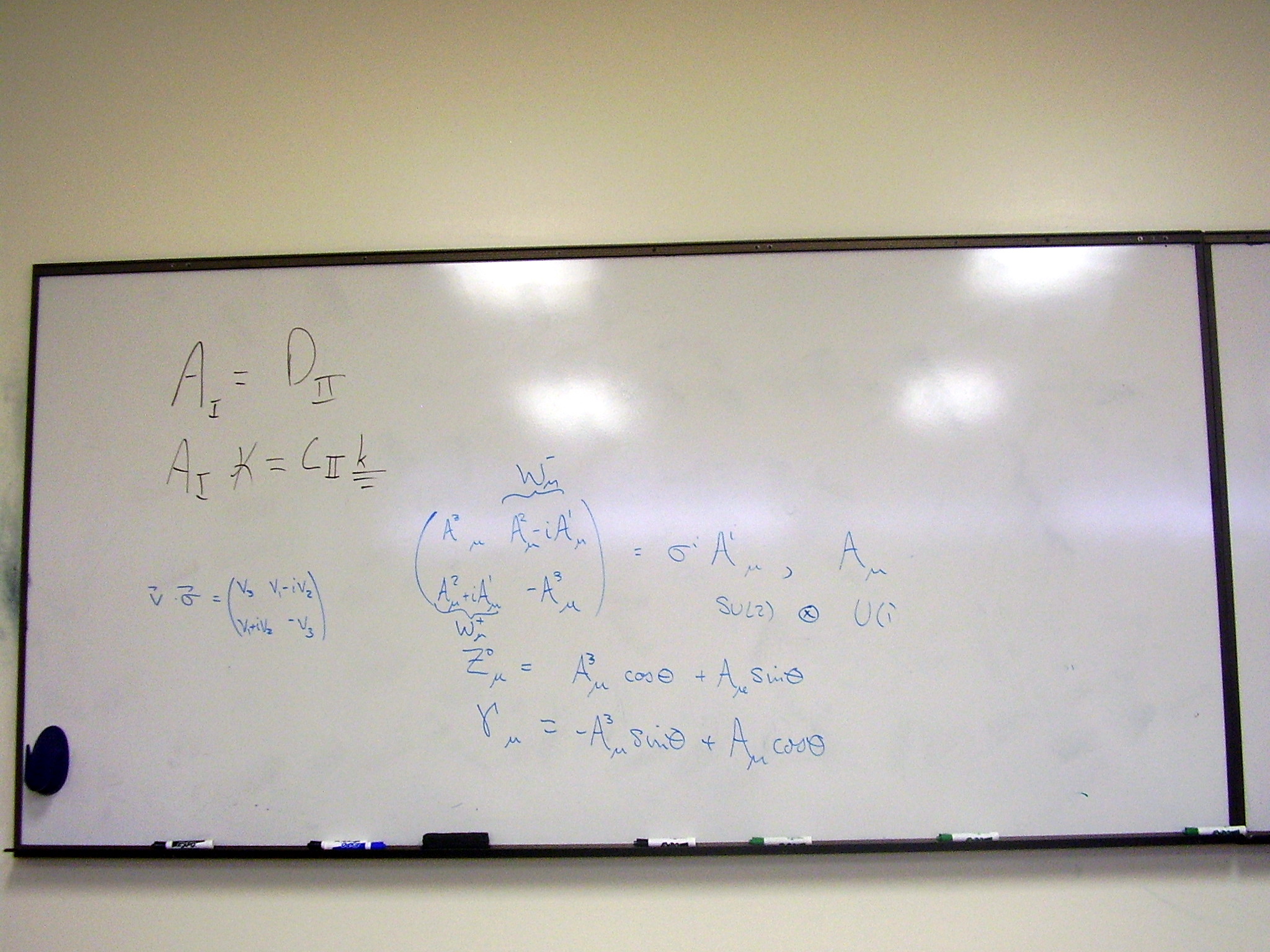
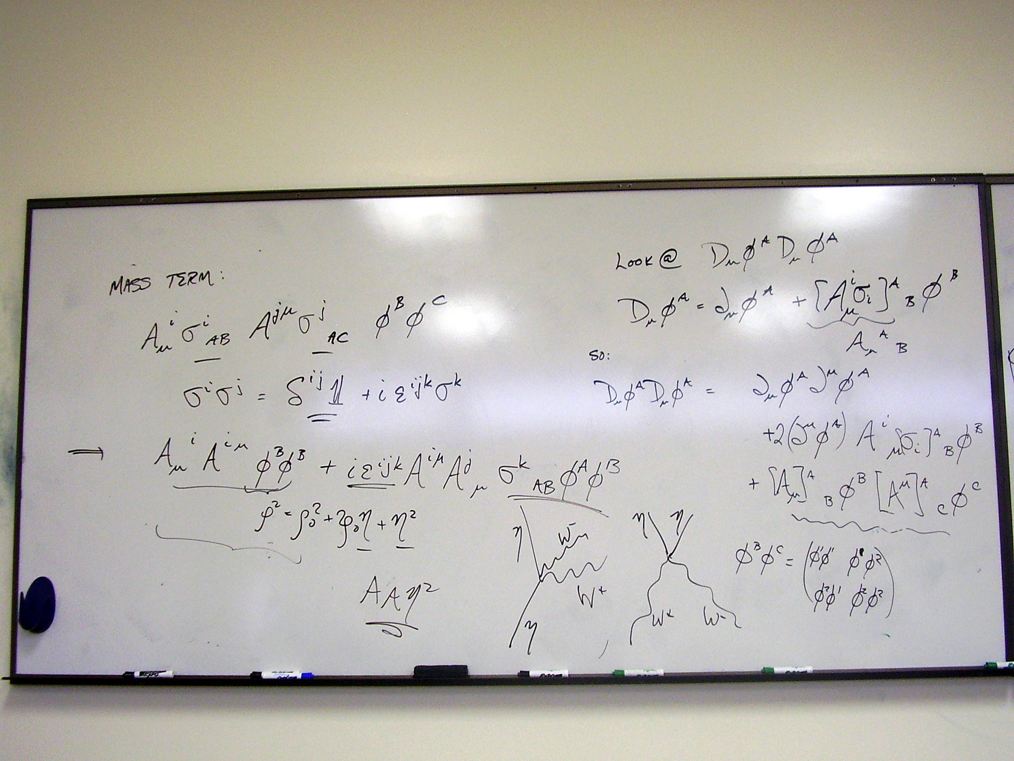
The problem of masses in
SU(2) (isospin) gauge theory: the gauge bosons are massless.
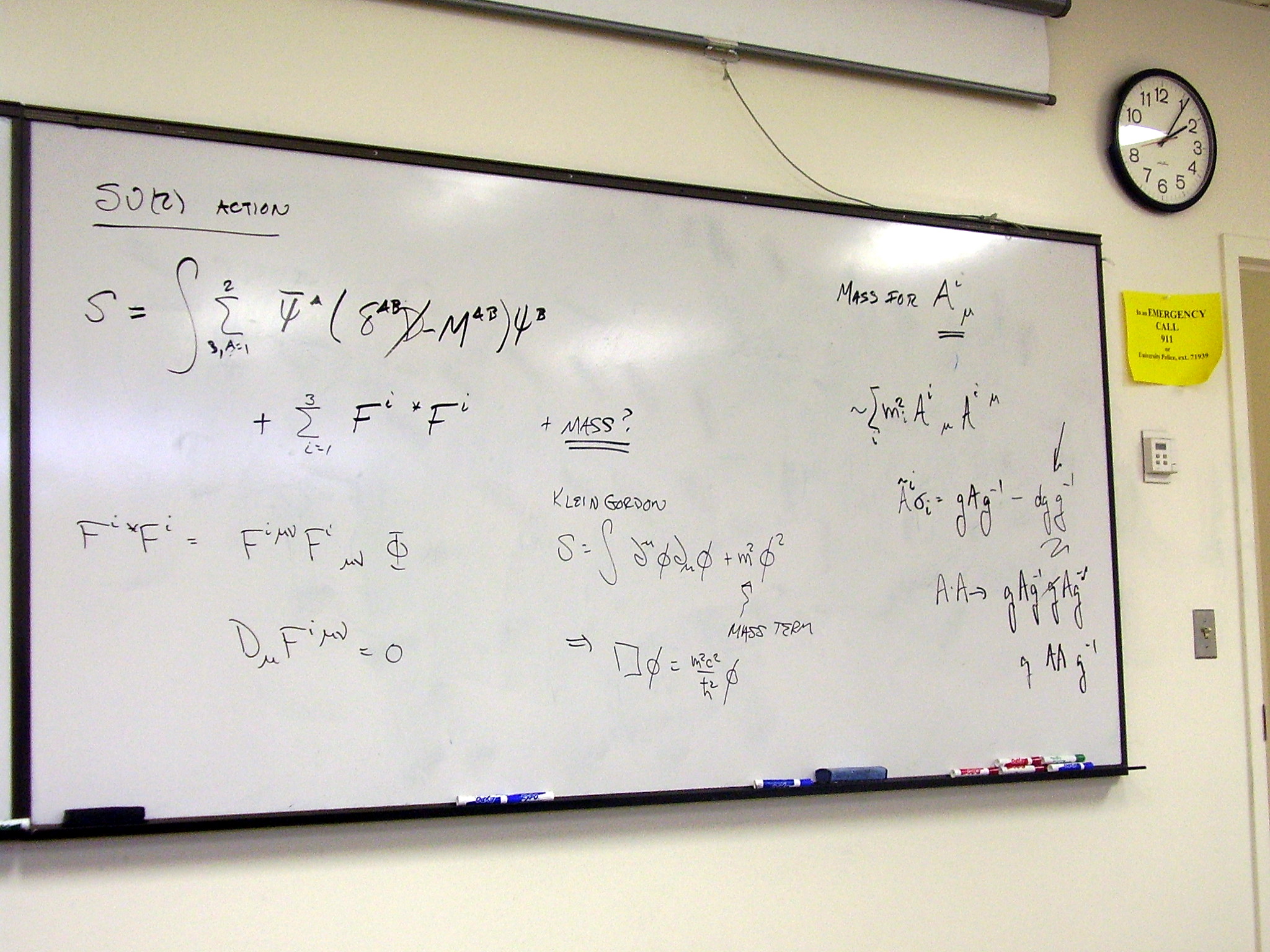
A potential solution via a
coupled scalar doublet, the Higgs particle.
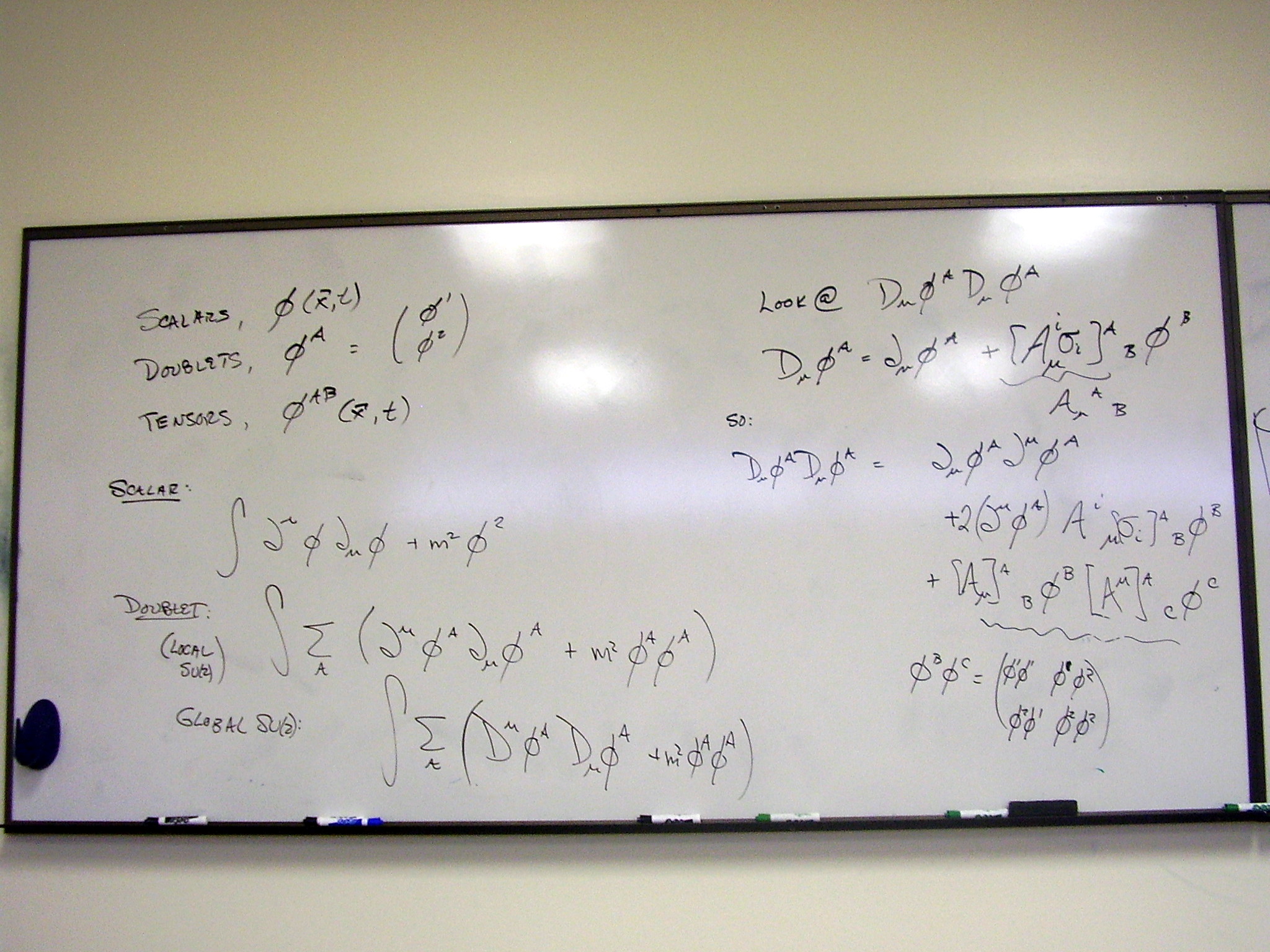
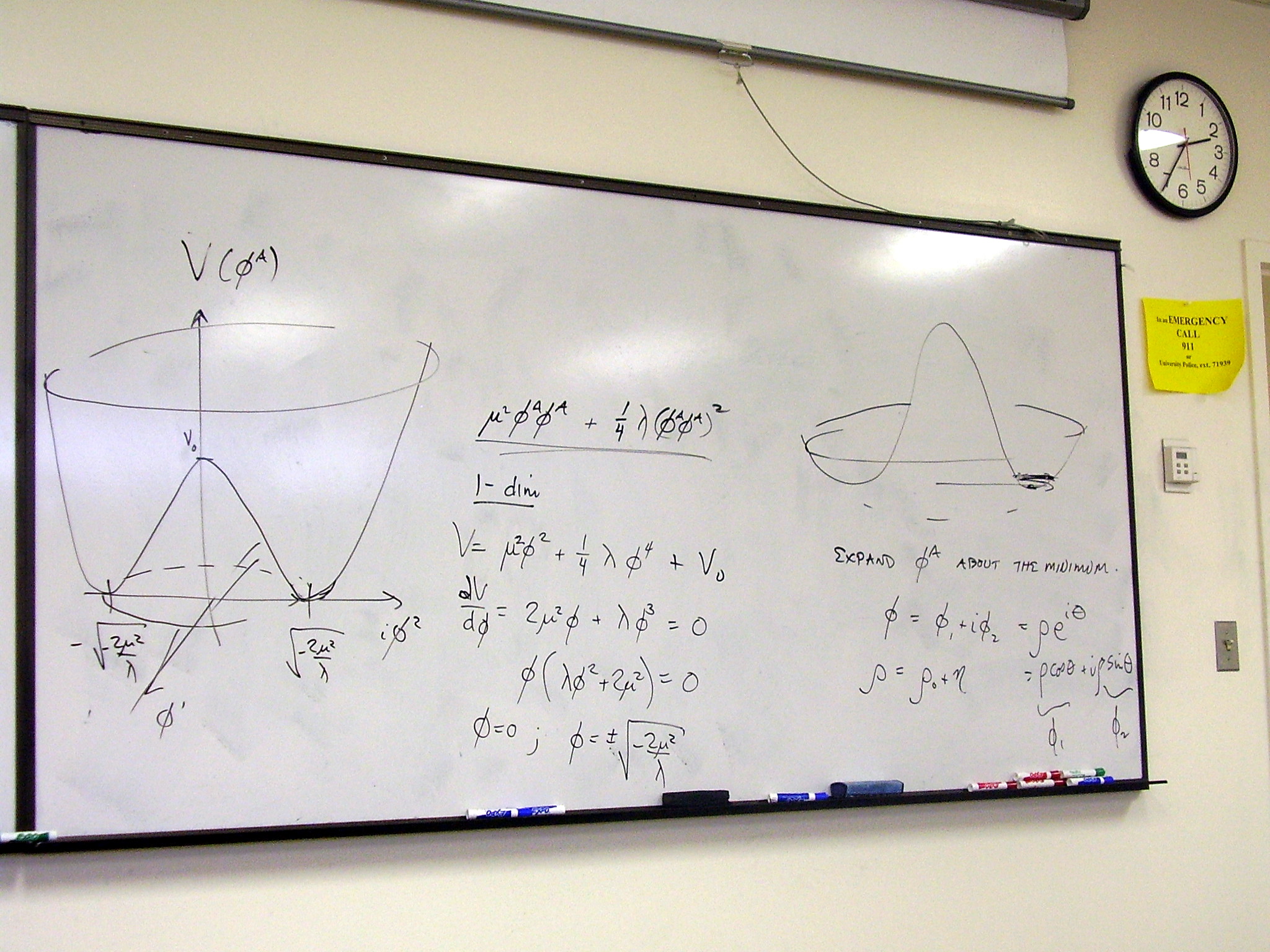
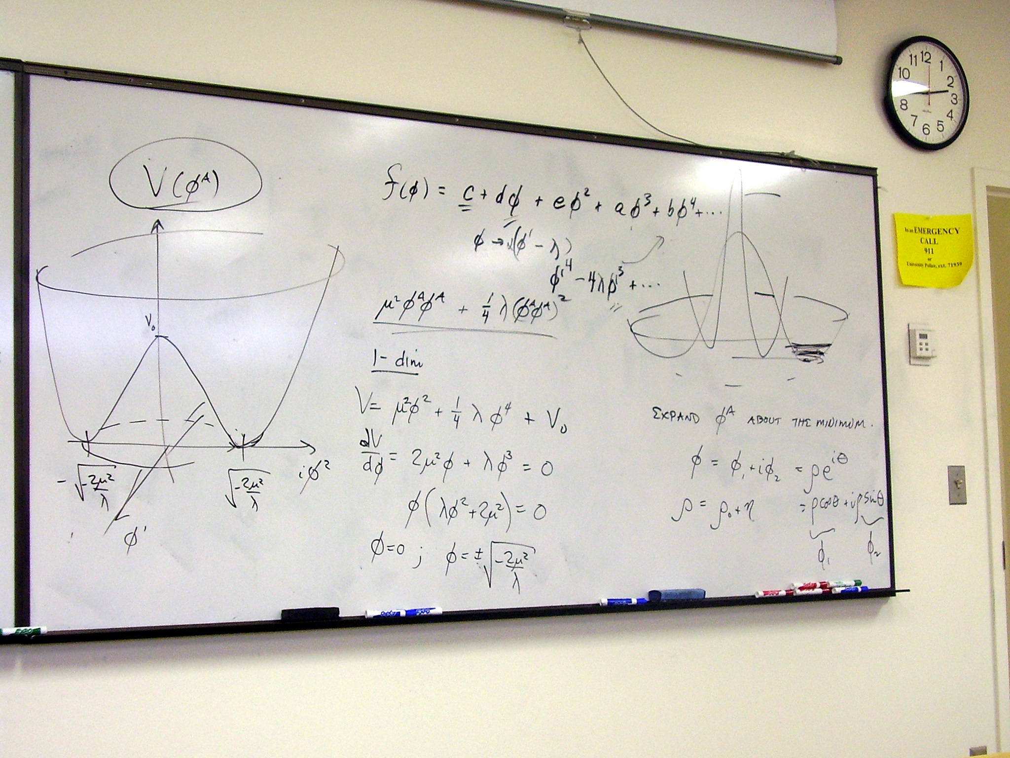
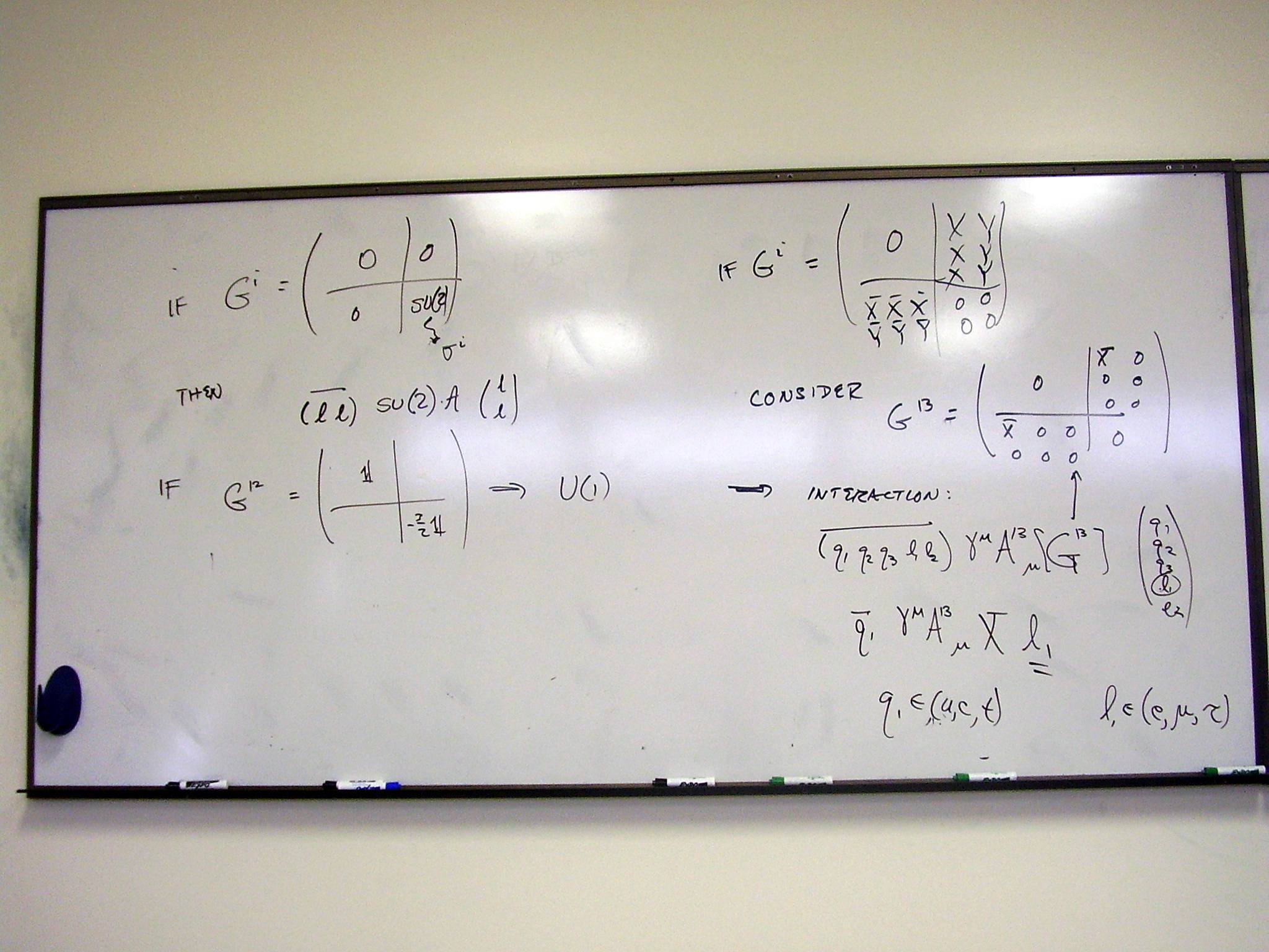
A Grand Unified Theory
(GUT) using SU(5). SU(5) contains the standard SU(3) x SU(2) x U(1) model with
the obvious embedding of SU(3) and SU(2). The traceless linear combination of
the 3 x 3 identity and the 2 x 2 identity generates U(1). Six new particles
(X,Y), called leptoquarks, are predicted by the model. These allow (too much)
baryon decay.
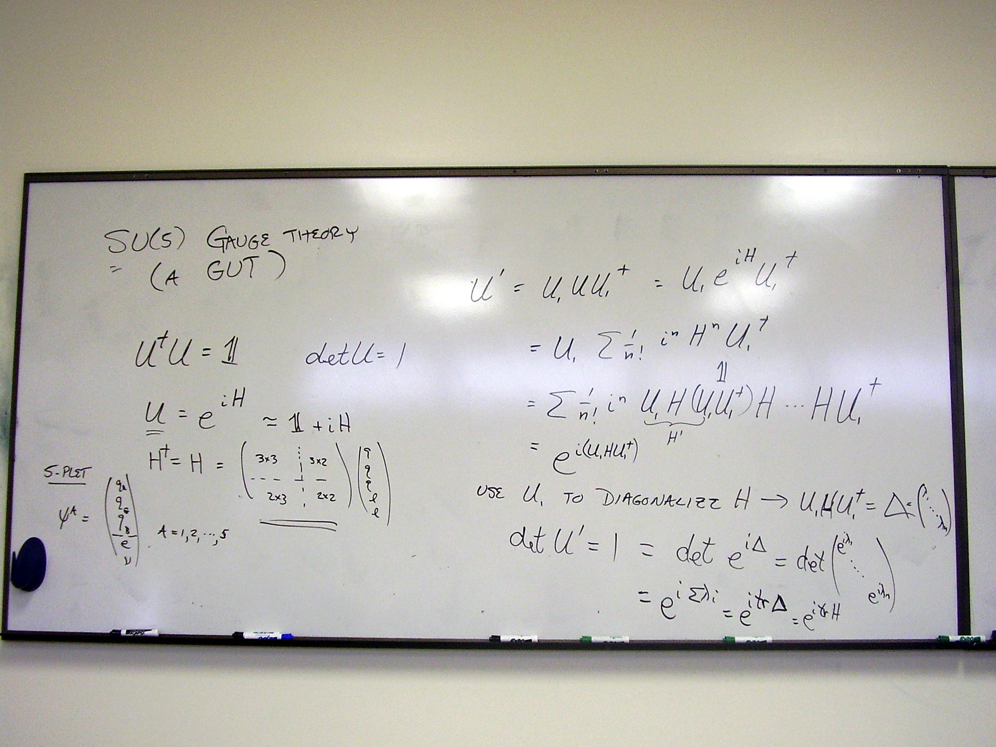
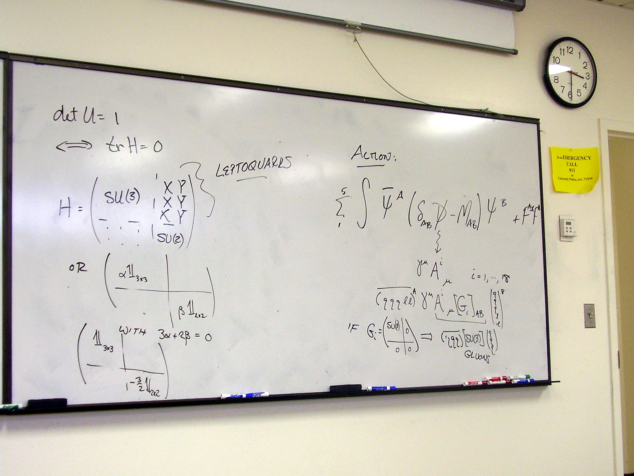
Friday, March 20, 2009
Lecture:
General relativity as a Poincaré gauge theory
Exercise: Gauge SU(3)
Steps in gauging the
Poincaré group
Linear representation;
infinitesimal generators
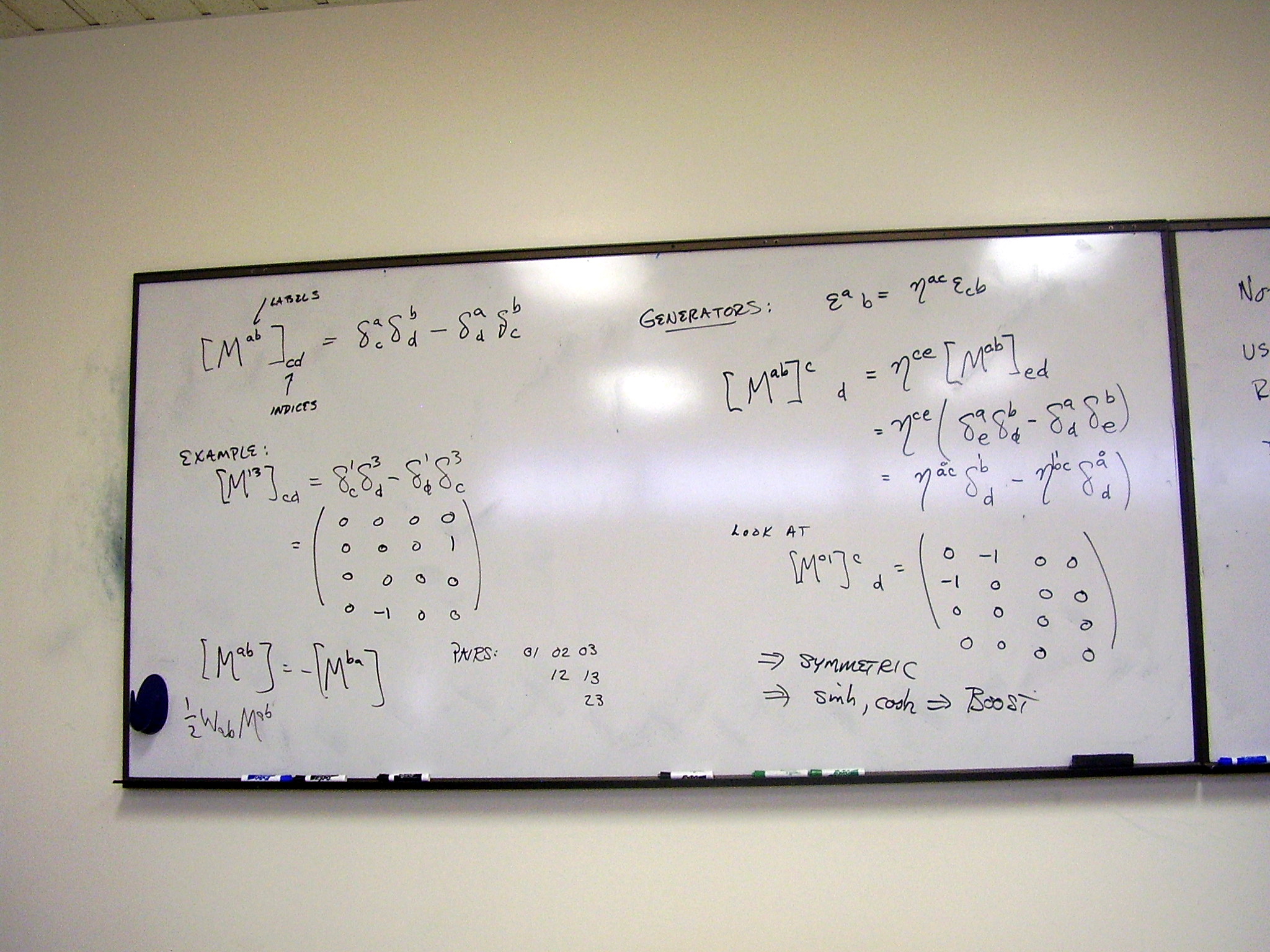
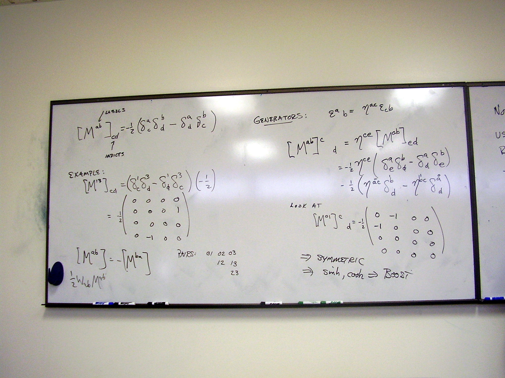
A basis for the Lie algebra
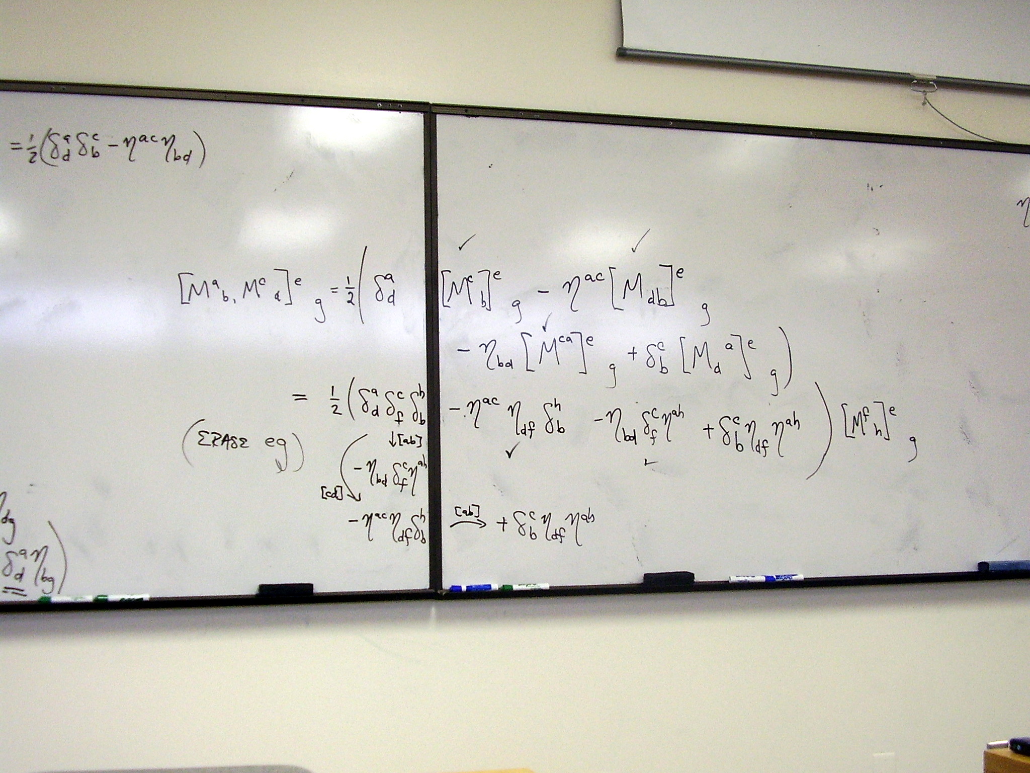
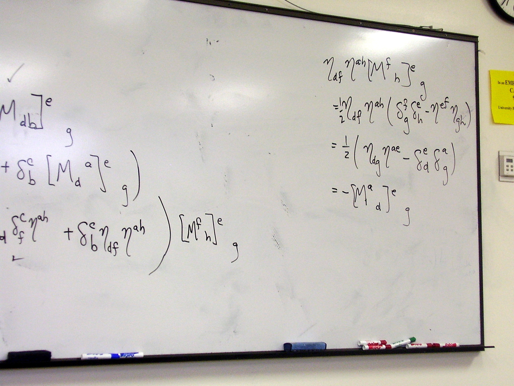
The Lie algebra of the
Lorentz generators (and, in fact, of SO(p,q))
Rearranging indices and
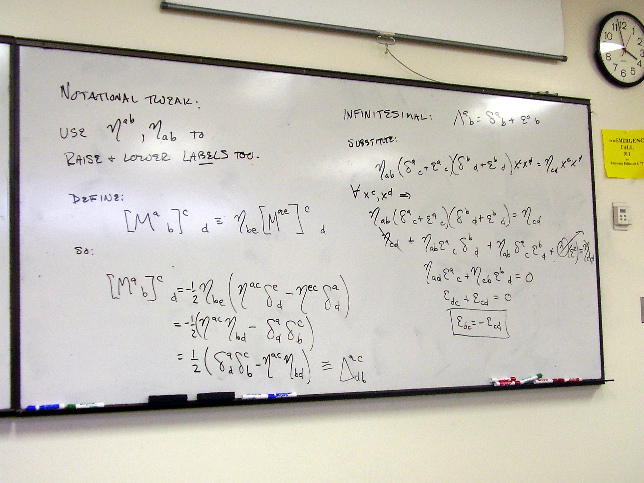
labels on the generators:
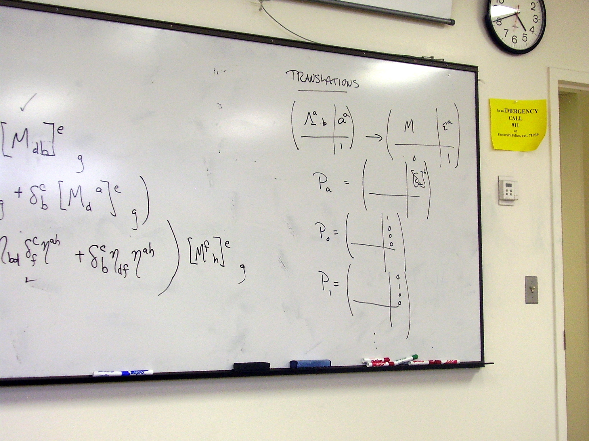
The translations:
Rotations (boosts) and
translations do not commute:
Defining dual 1-forms; the
Maurer-Cartan equations
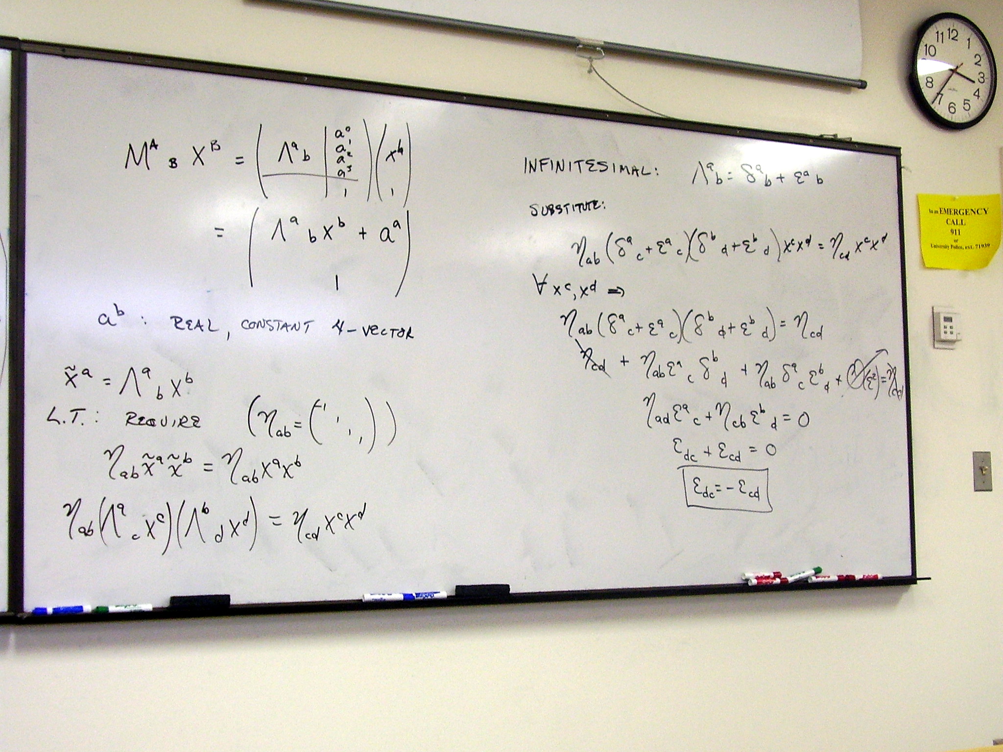
Monday, March 23, 2009
Lecture:
General relativity as a Poincaré gauge theory, continued
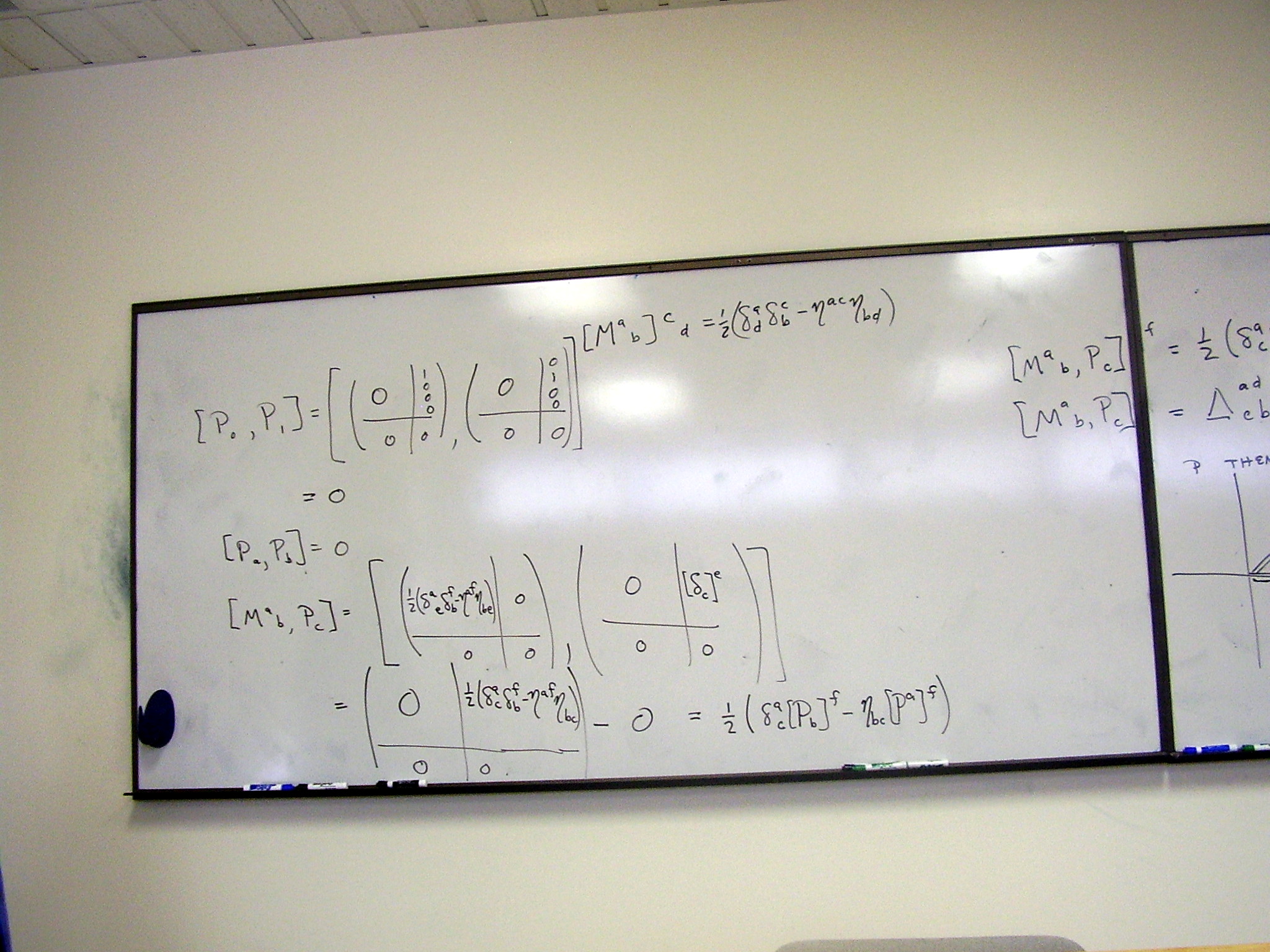
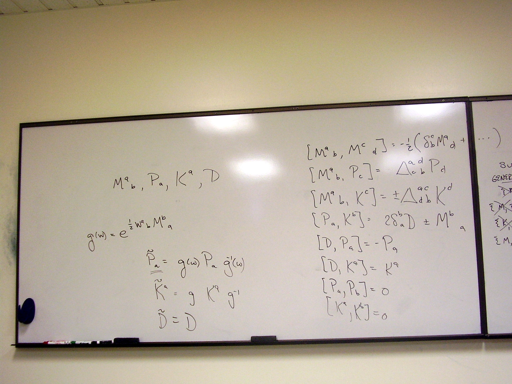
The Poincaré Lie algebra
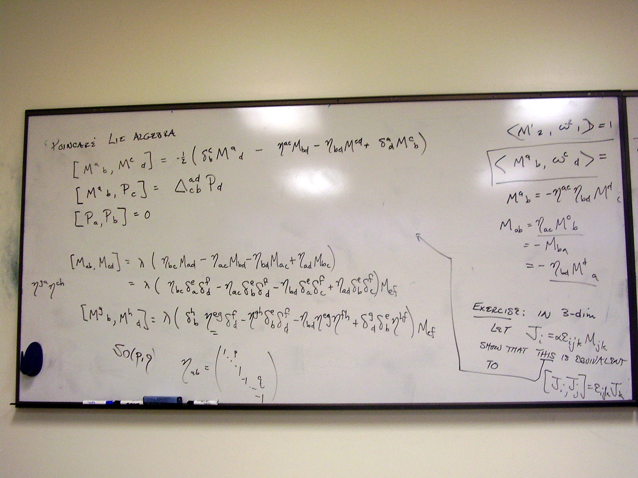
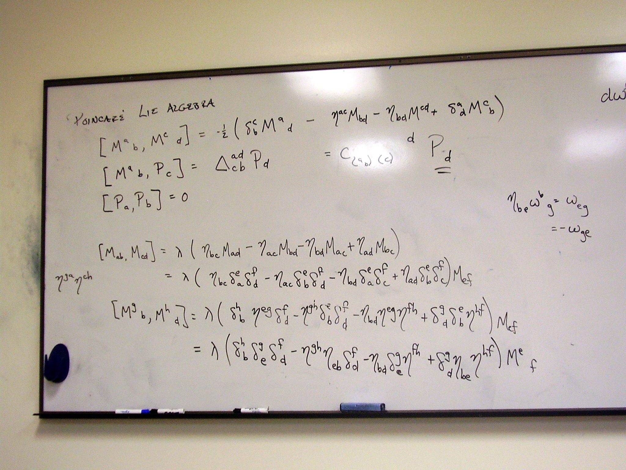
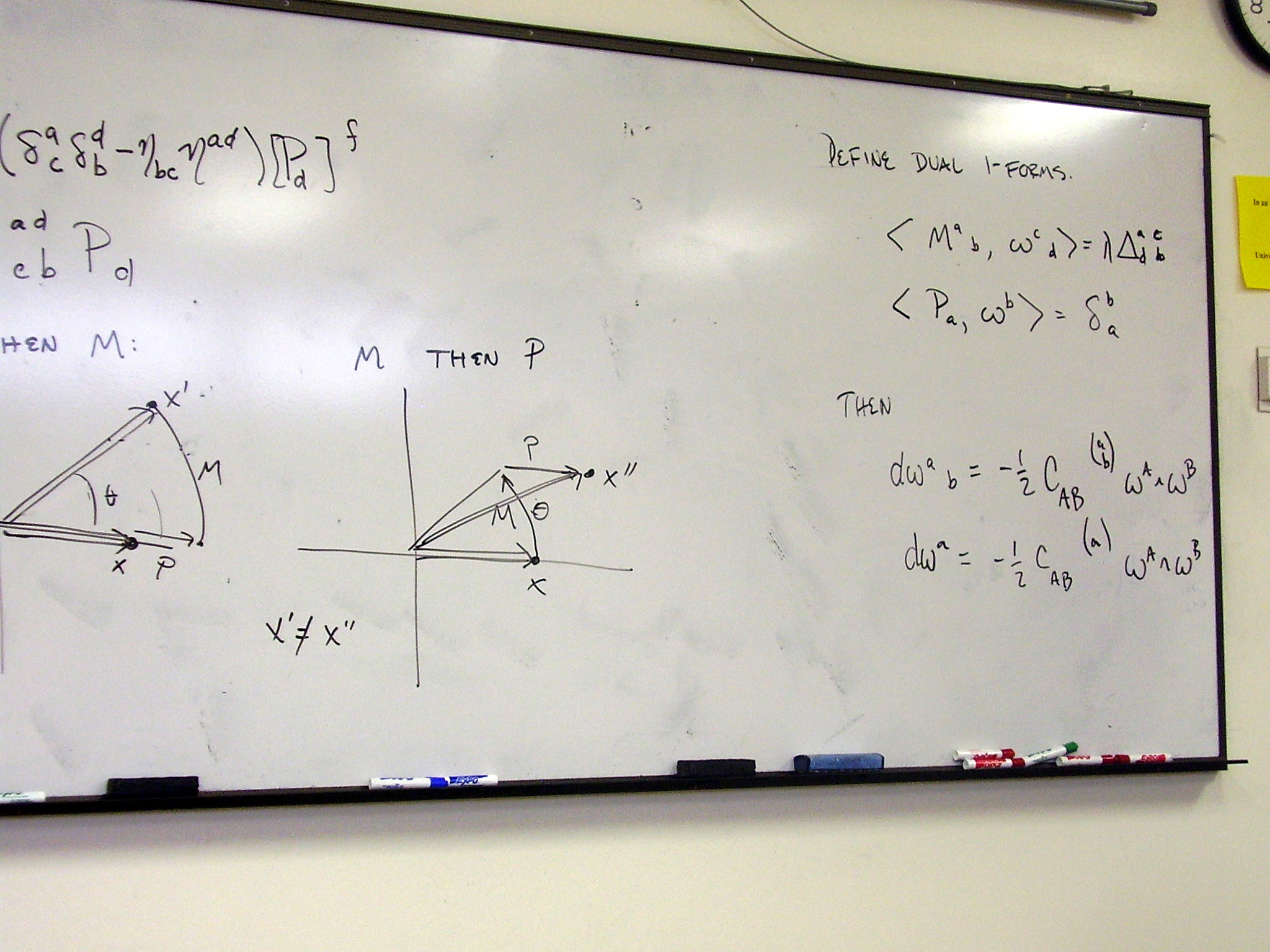
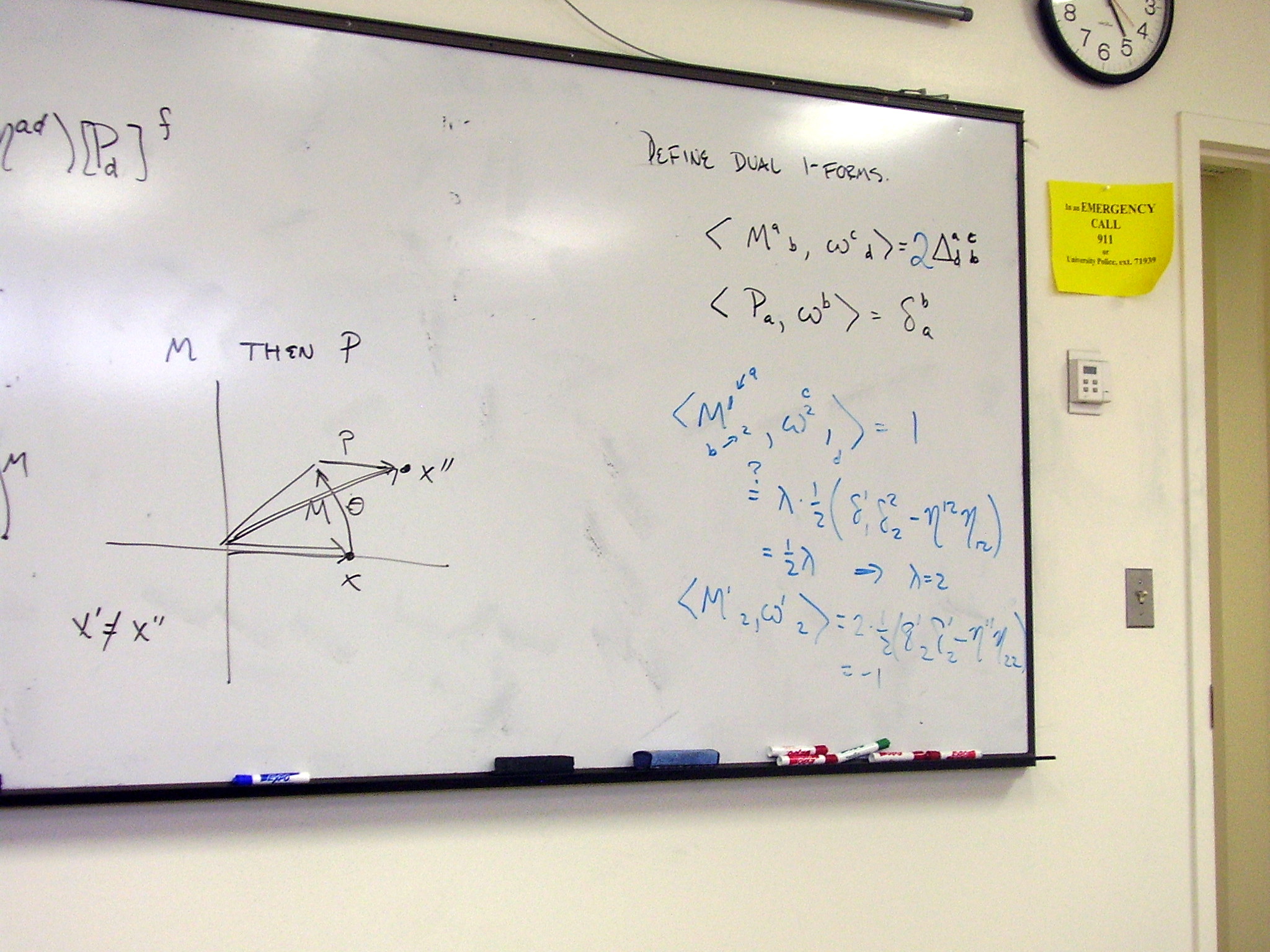
Dual 1-forms – the
Poincaré spin connection and solder form
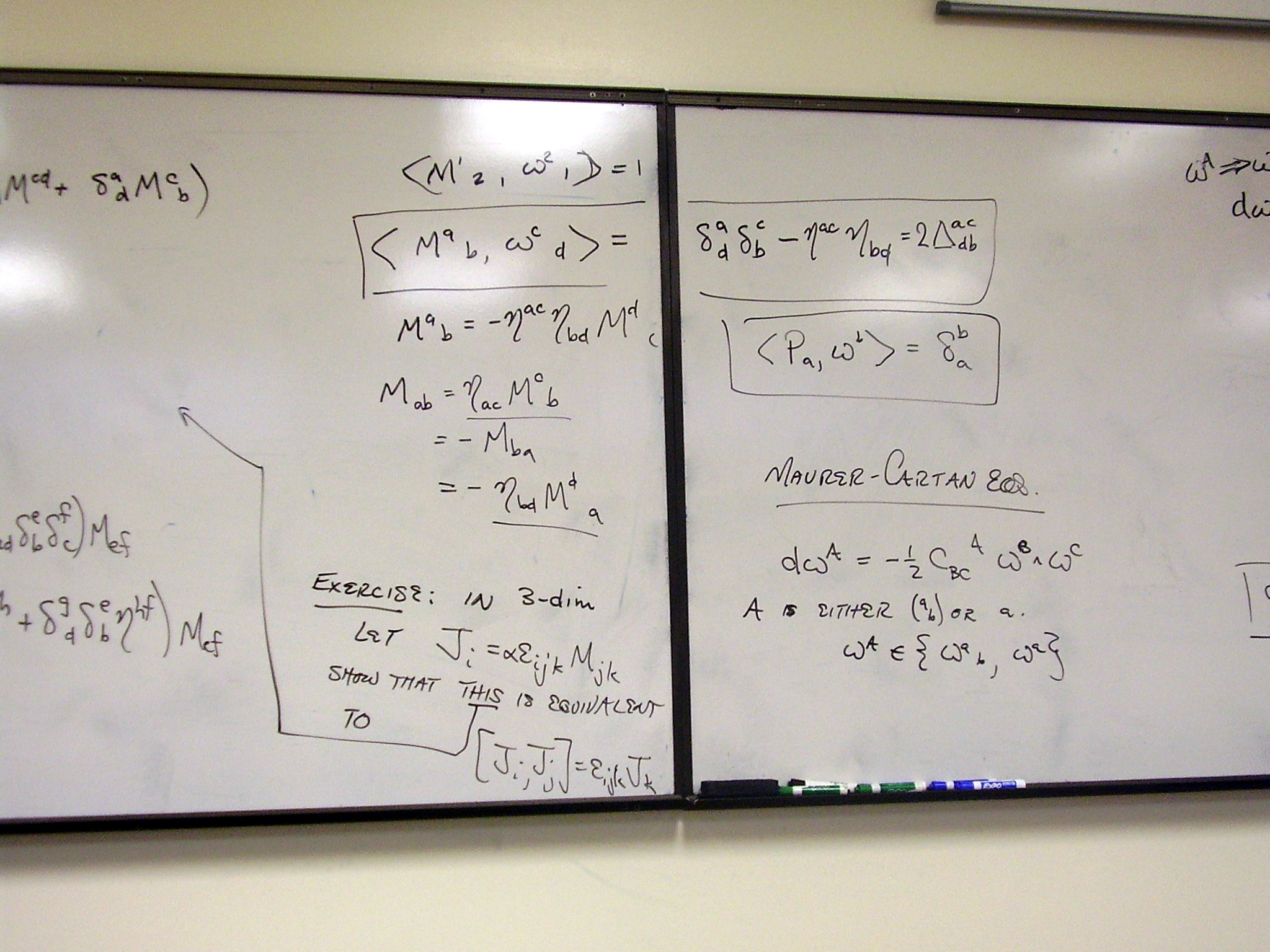
Maurer-Cartan structure
equation for the solder form:
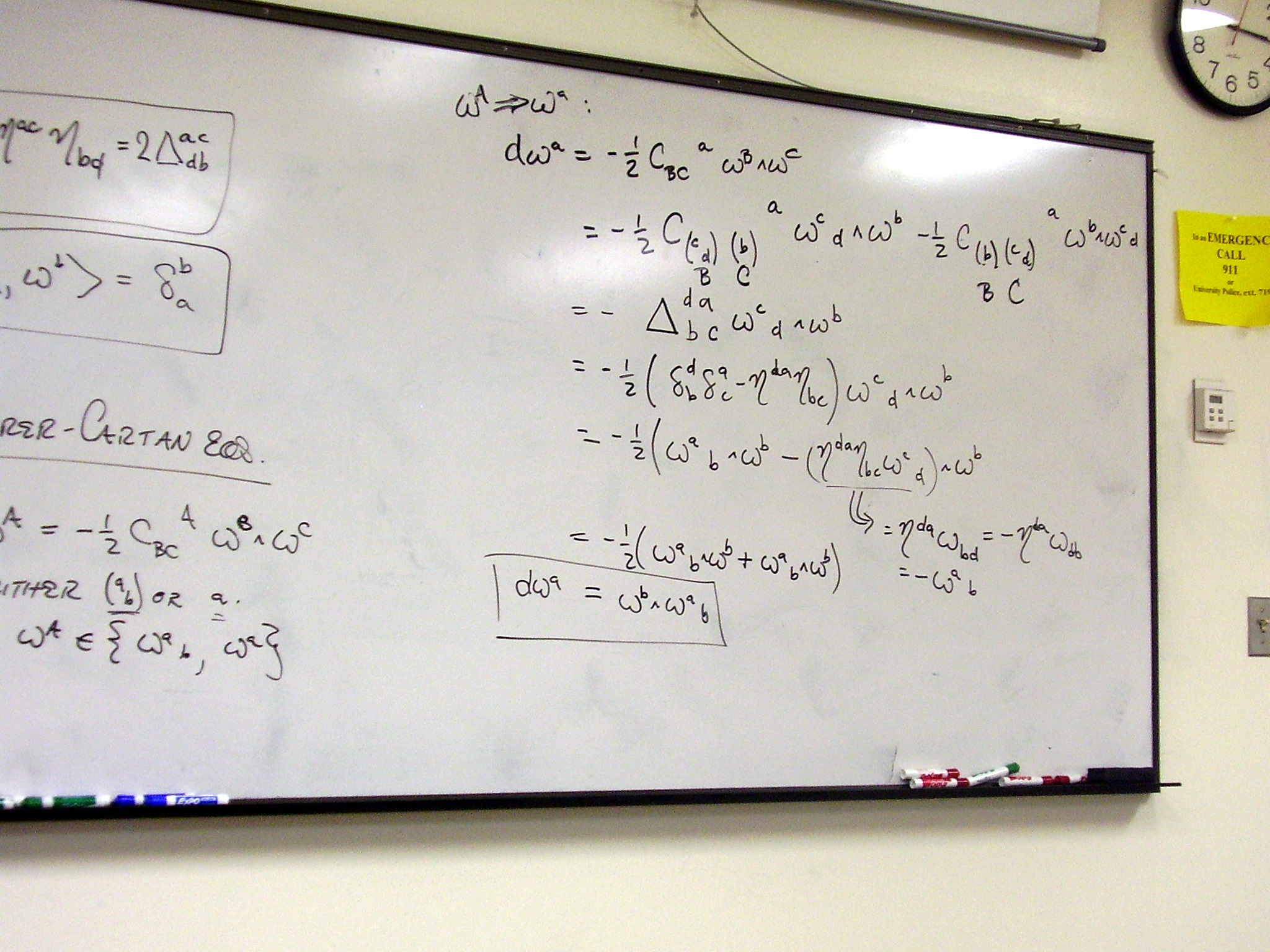
Maurer-Cartan structure
equation for the spin connection (and ANY SO(p,q) connection!):
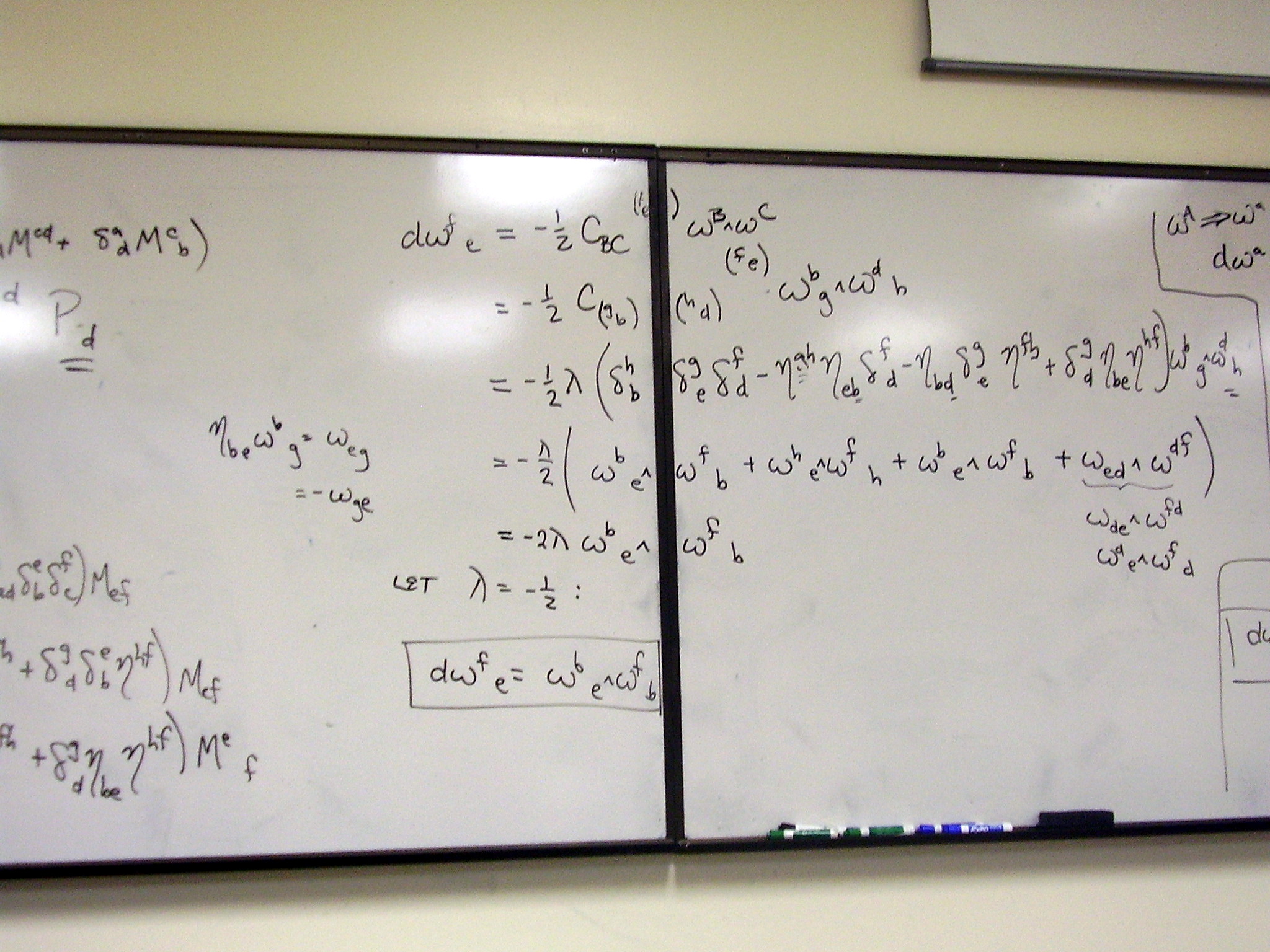
The Maurer-Cartan equations
for the Poincaré group. The next steps: the group quotient and generalization
of the connection to give curvature 2-forms. Form of the curvatures.
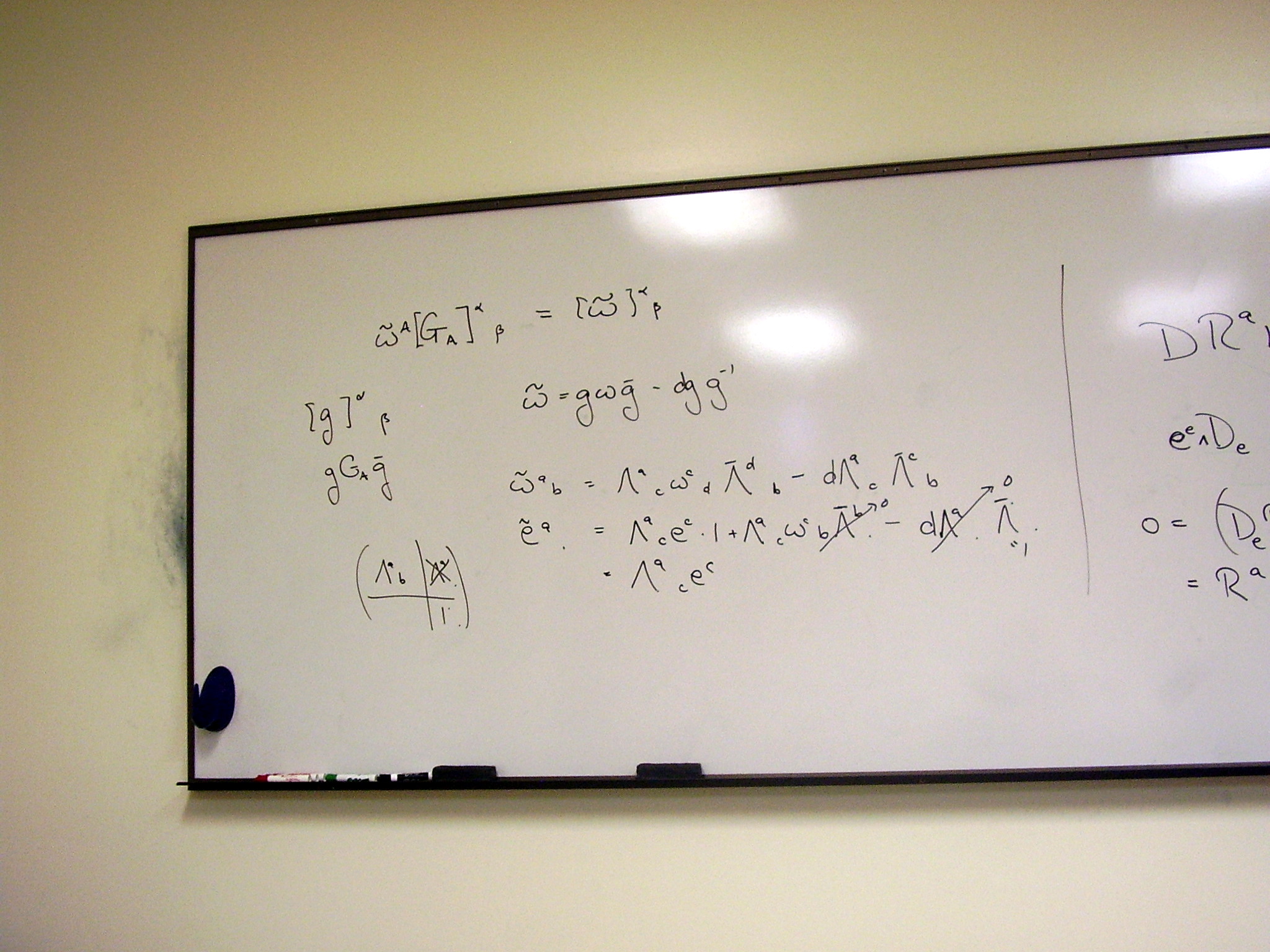
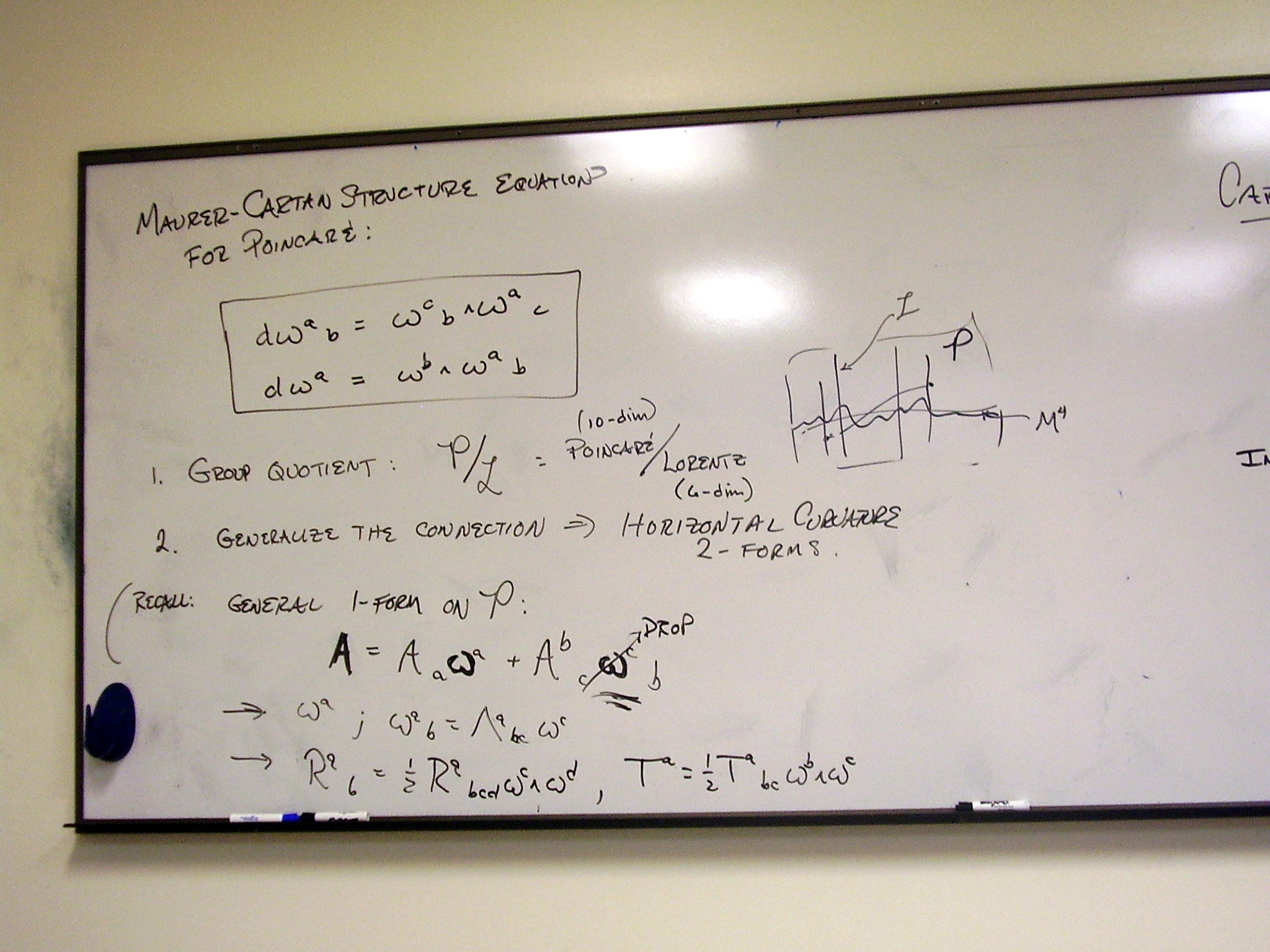
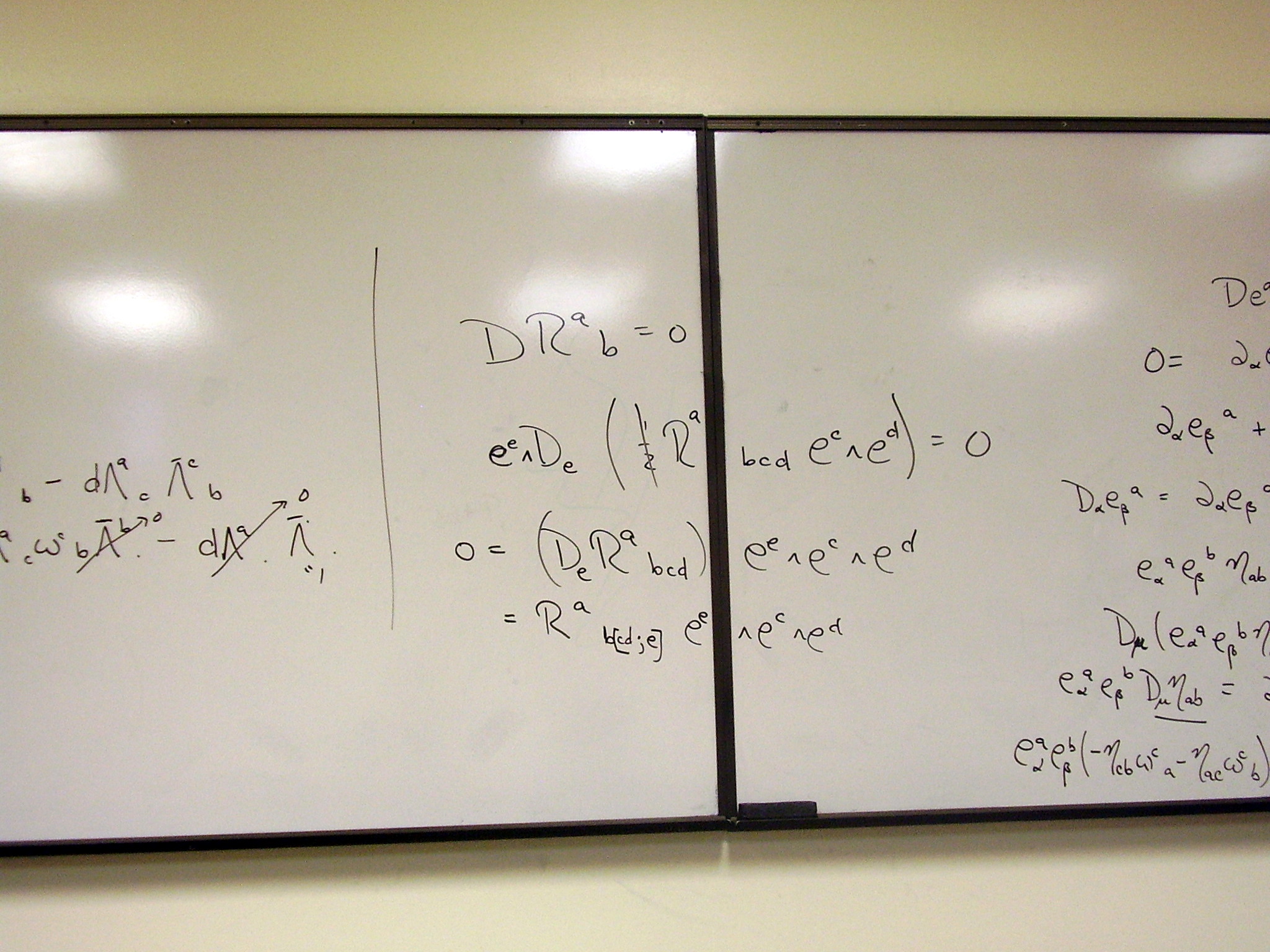
The Cartan structure
equations for the Poincaré group, and their Bianchi identities:
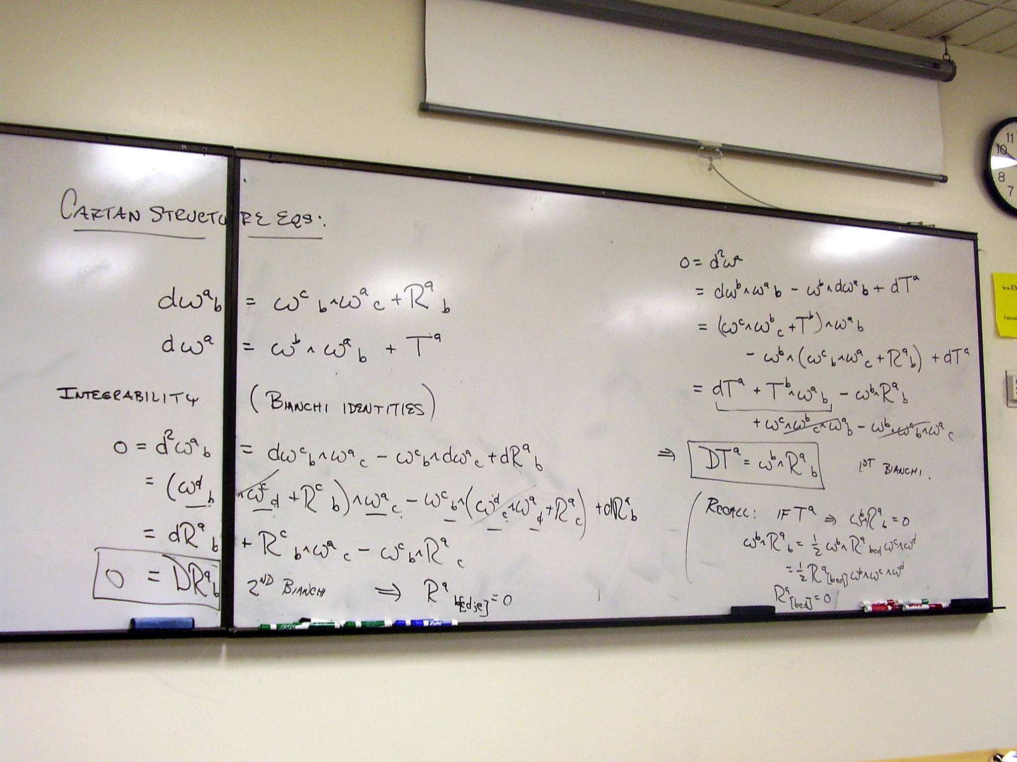
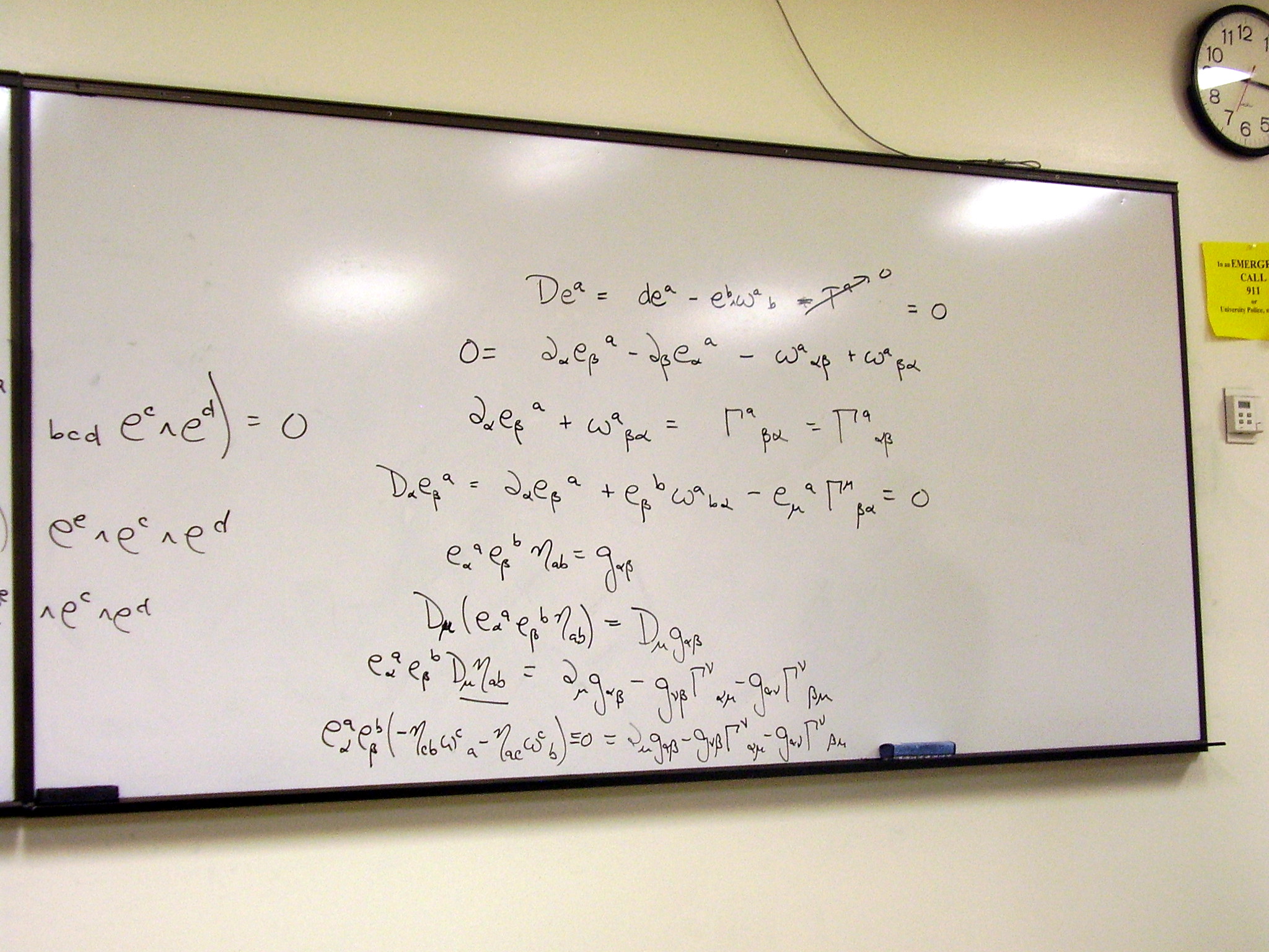
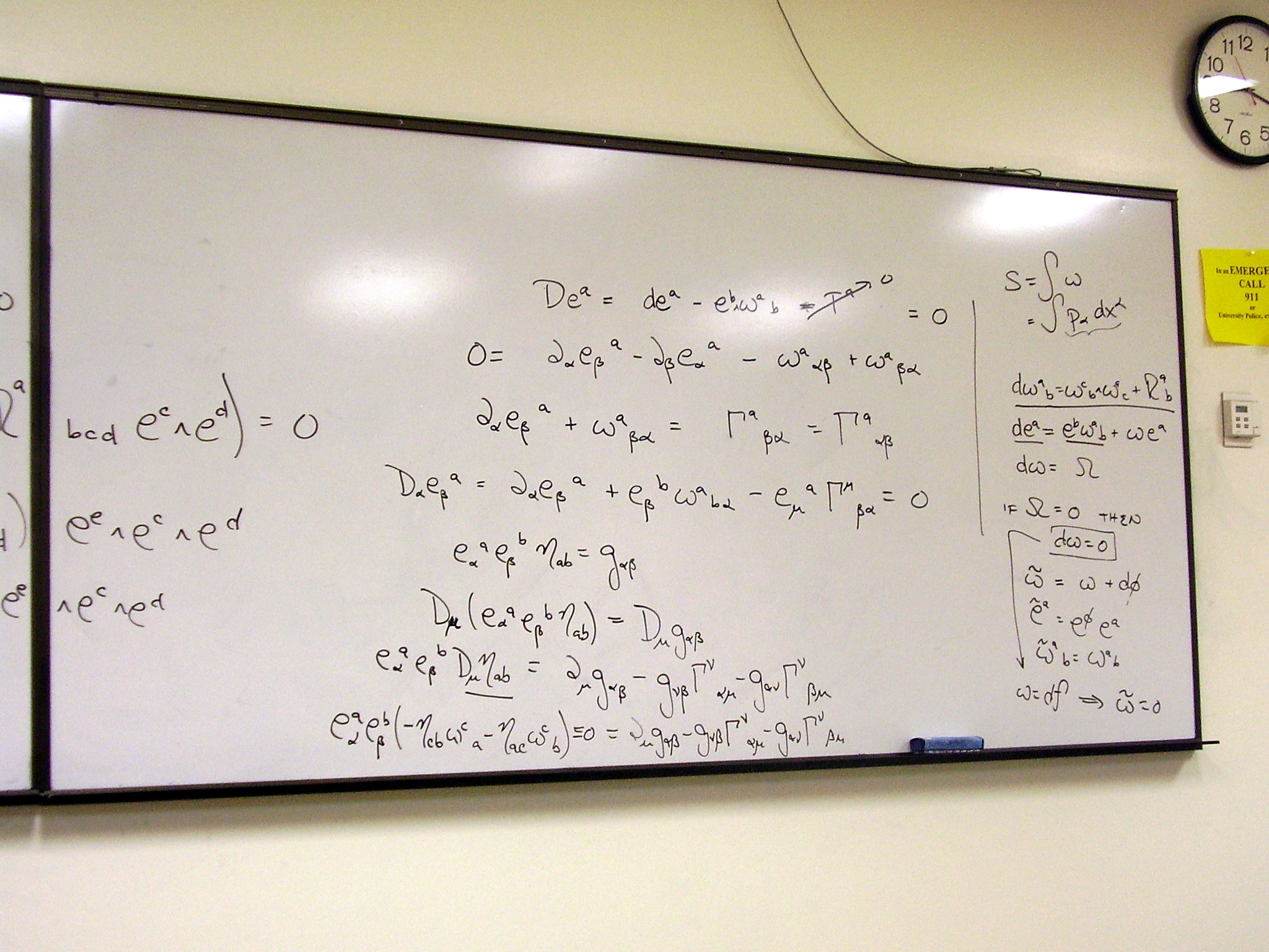
The solder form as
orthonormal frame field. Tensors of the Poincaré gauging.
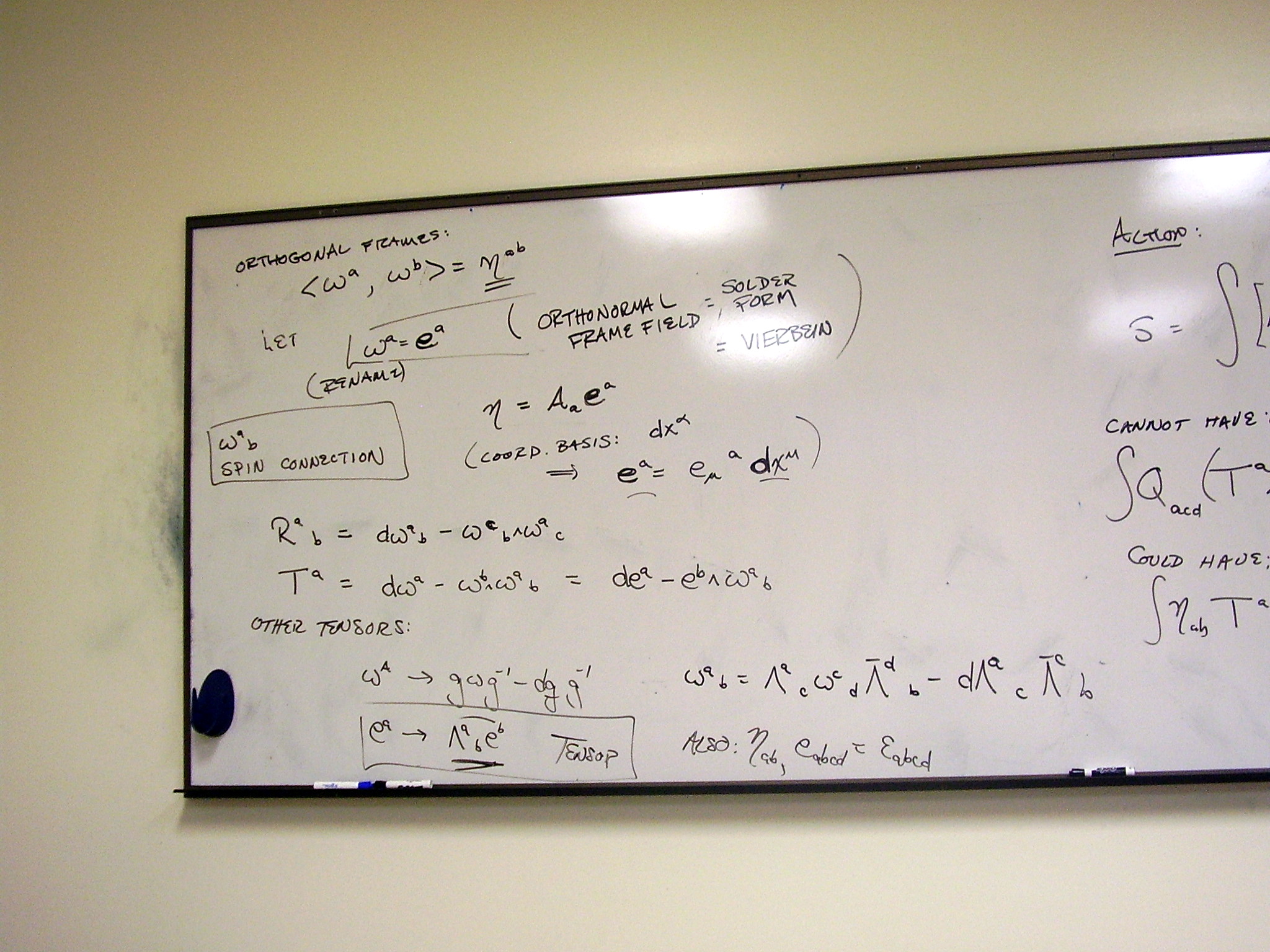
General action for Poincaré
gauge theory:
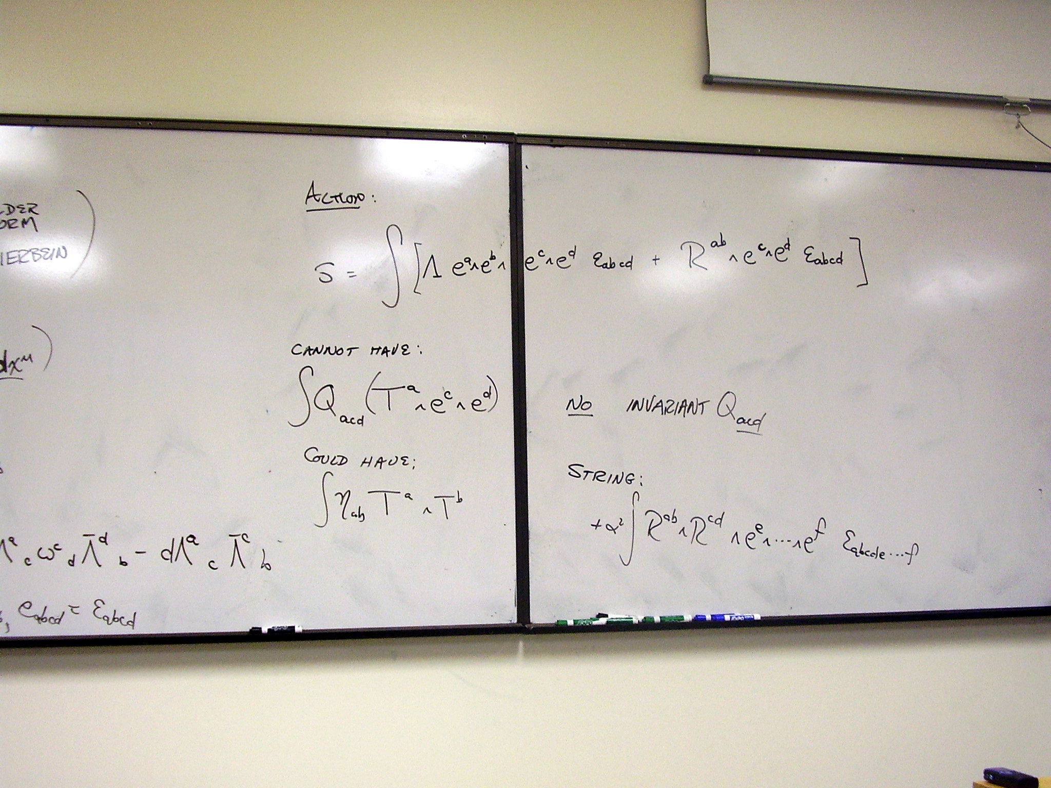
Varying the action: the Einstein equation with cosmological
constant
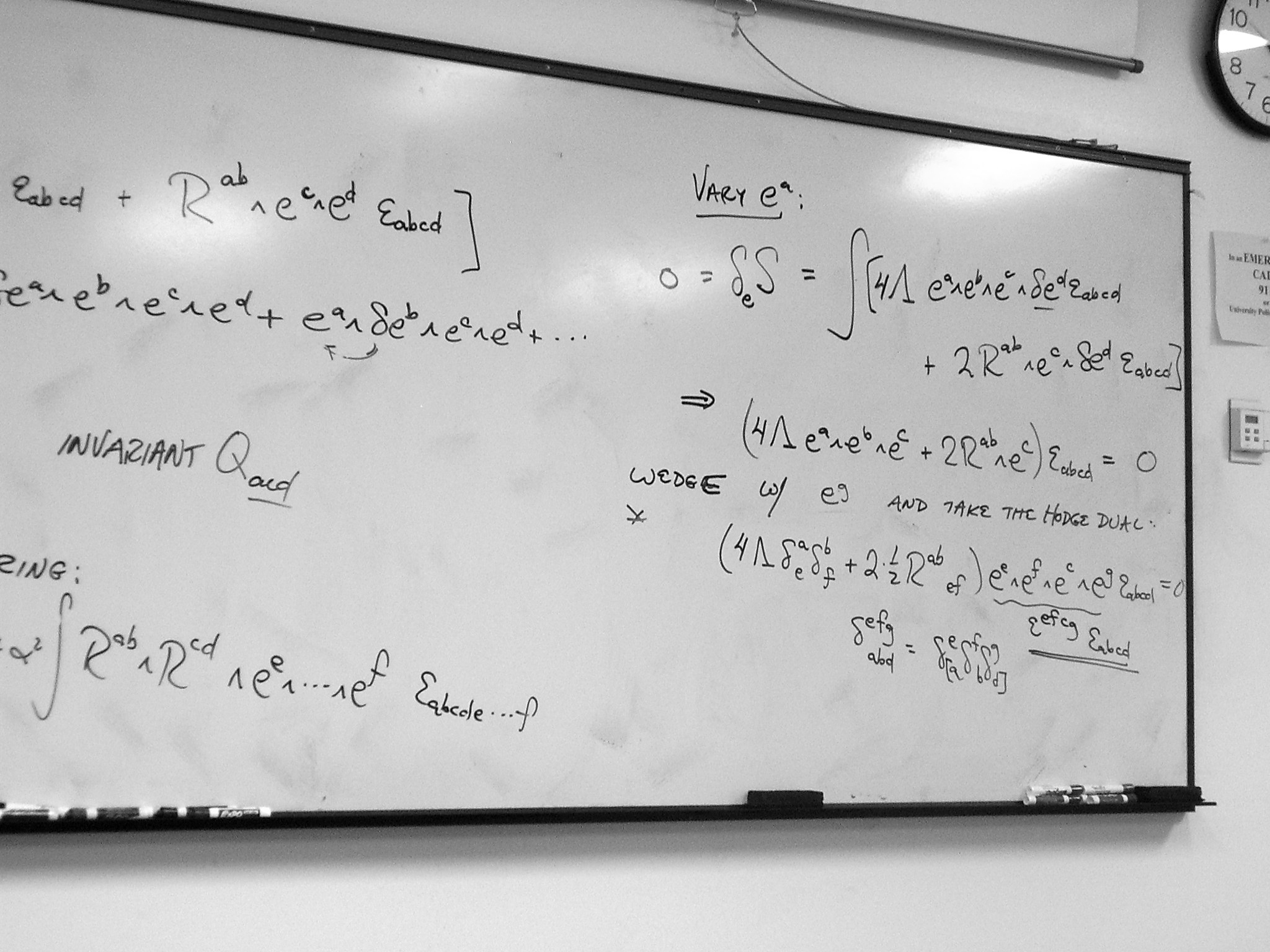
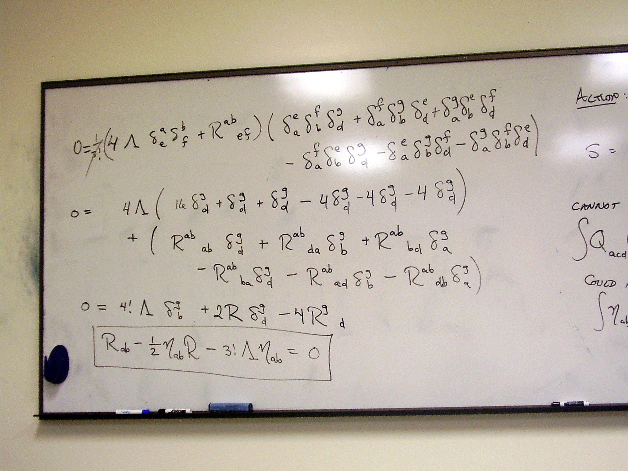
Notes: March 27 -
April 3
Notes: Conformal
generators and Maurer-Cartan equations
Monday, March 30, 2009
Lecture:
Beyond general relativity
Scale invariance and
non-Riemannian geometry
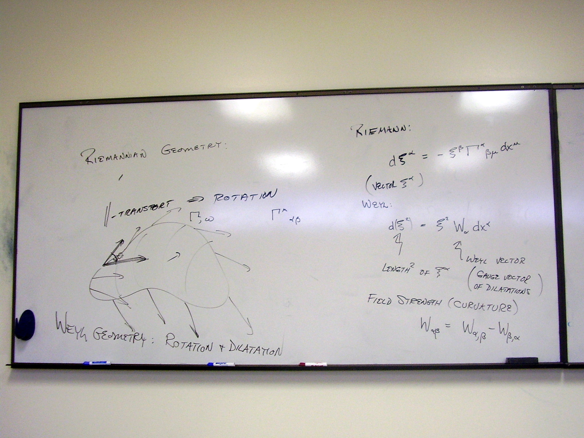
Geometry based on physical
measurements: Ehlers, Pirani & Schild. Possible symmetries for a
fundamental geometry
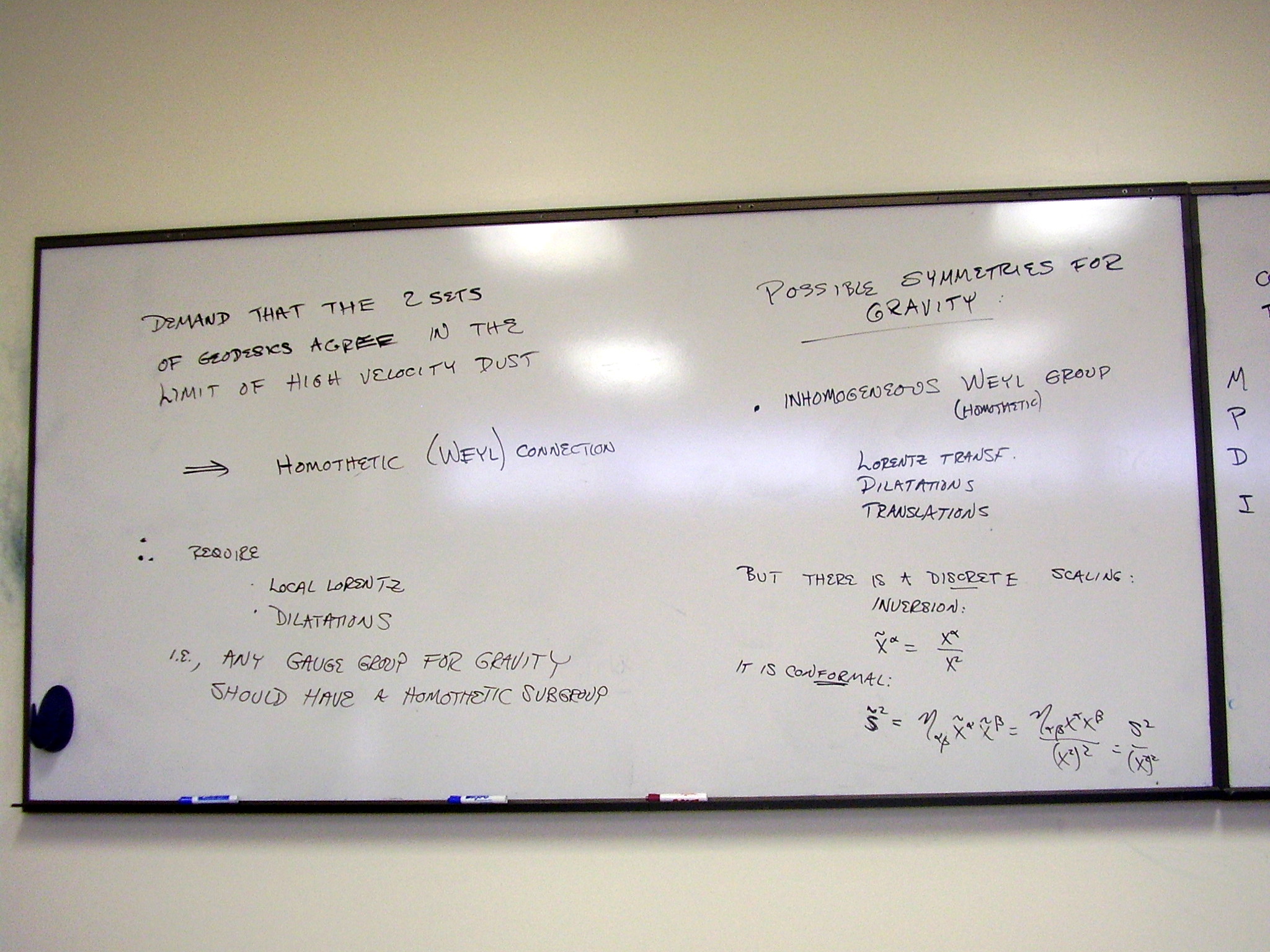
The spacetime conformal
group. SO(4,2)
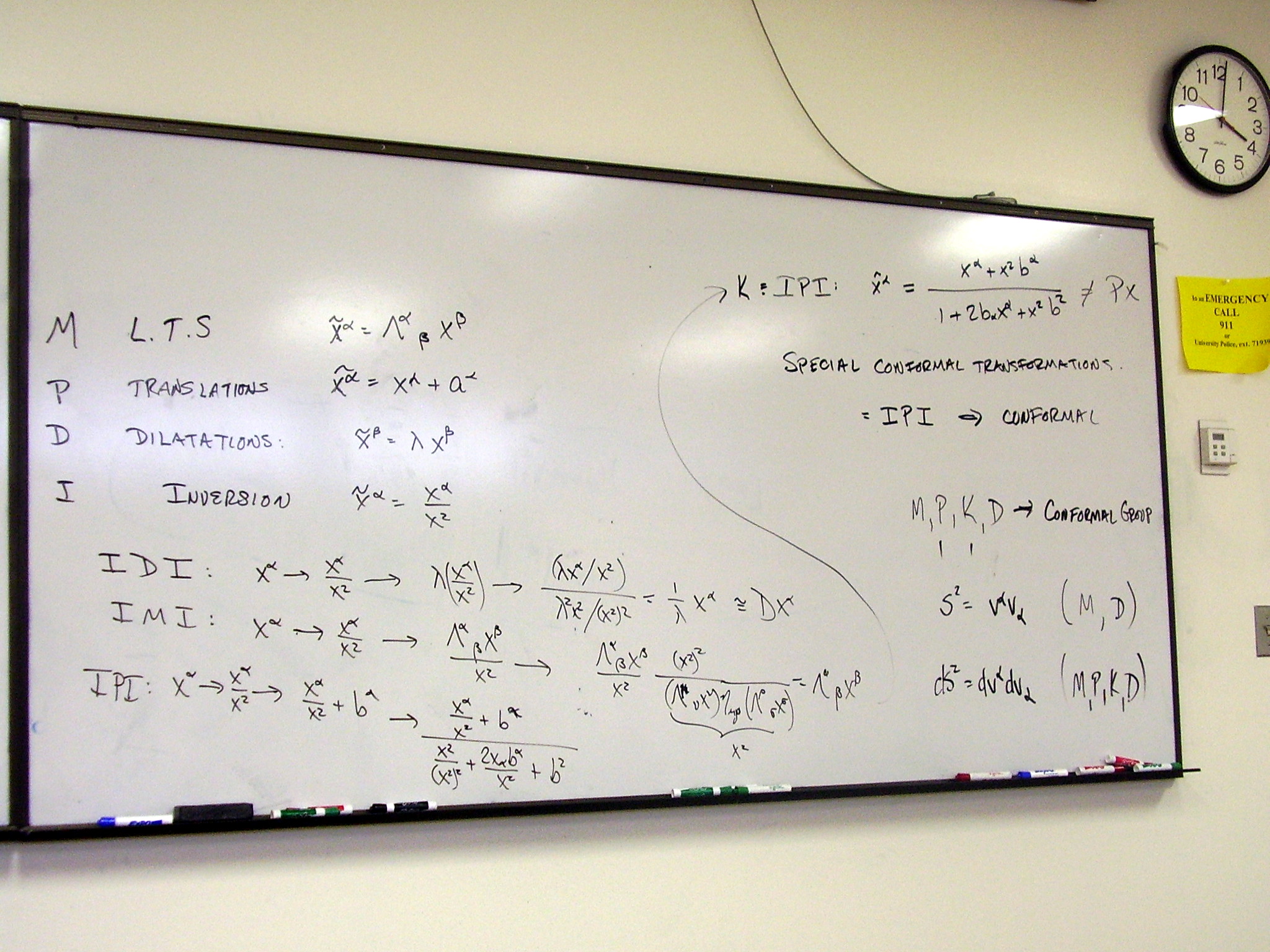
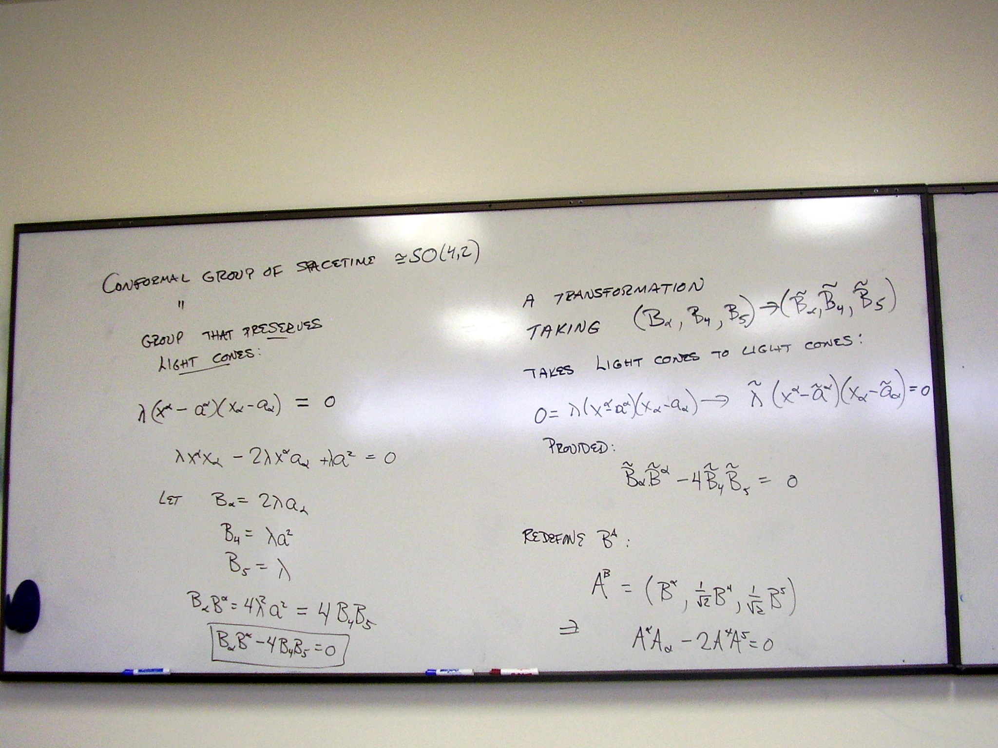
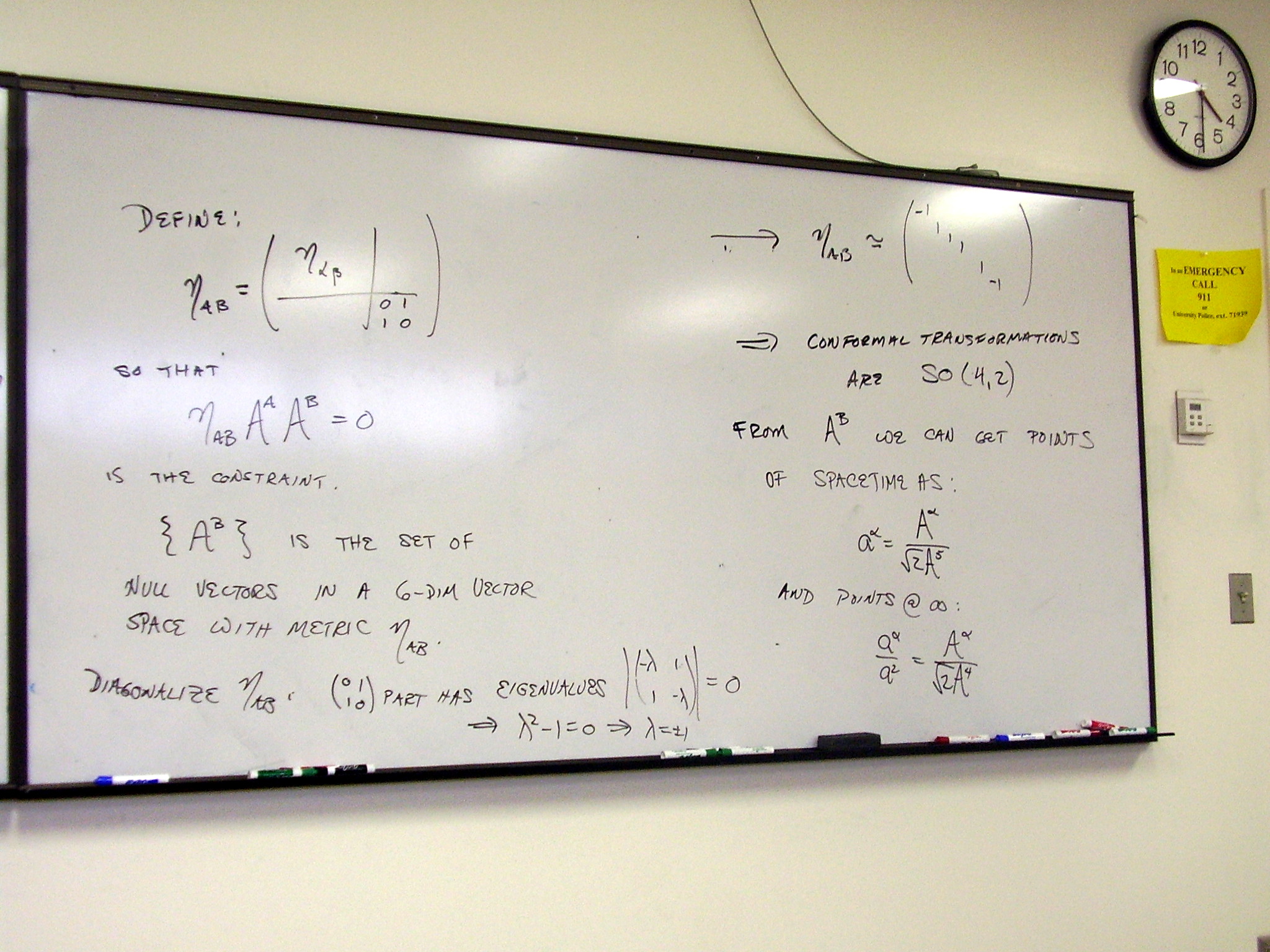
F-19 Flying Turtle
Wednesday, April 1,
2009
There’s some very silly
stuff in here!
Q: Where does the quotient
show up in the structure equations?
A: It doesn’t. It shows up
when we expand horizontal forms – the horizontal forms provide the basis.
Scenes from the Photo Shoot
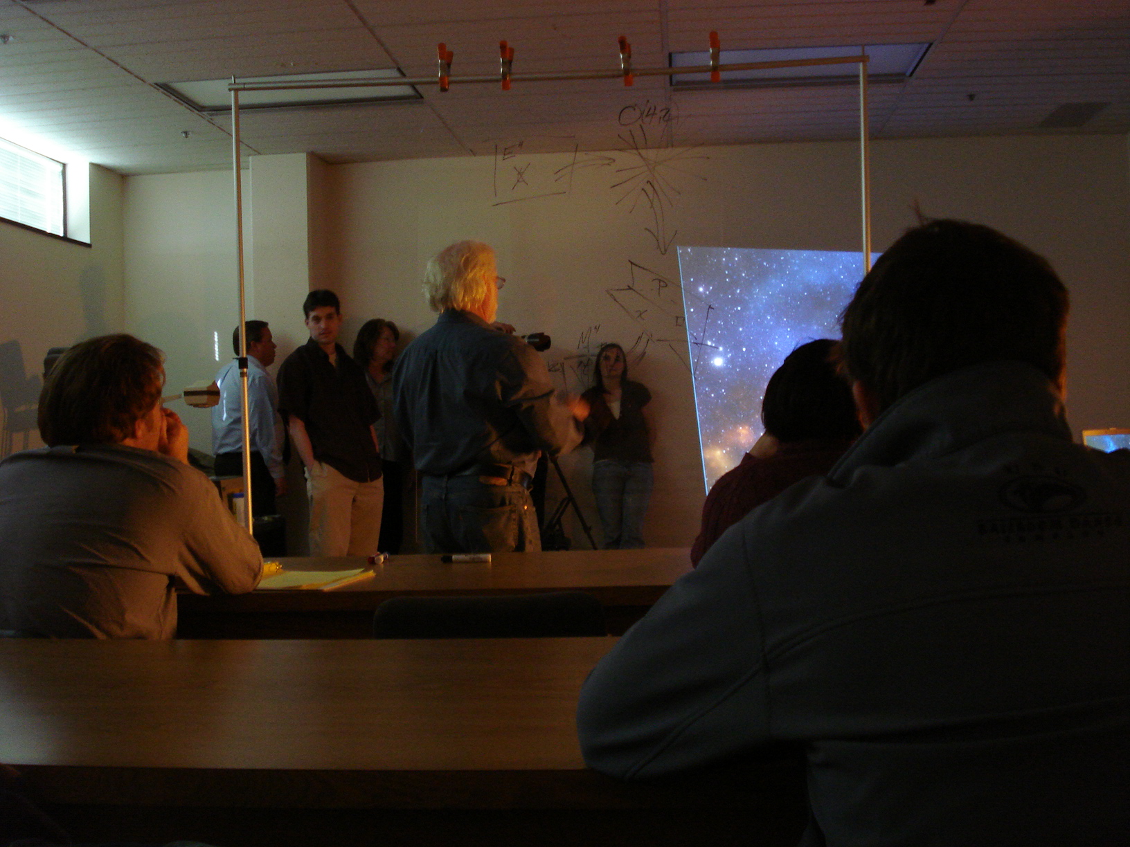
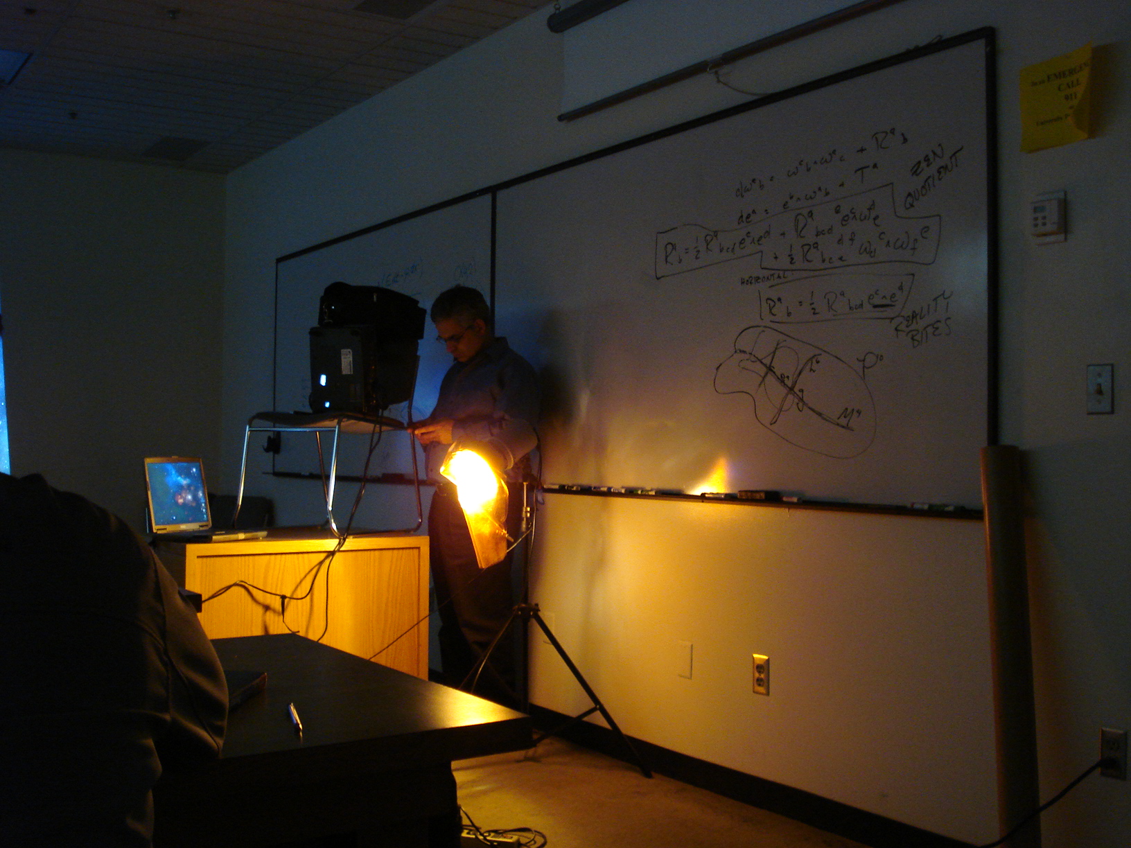
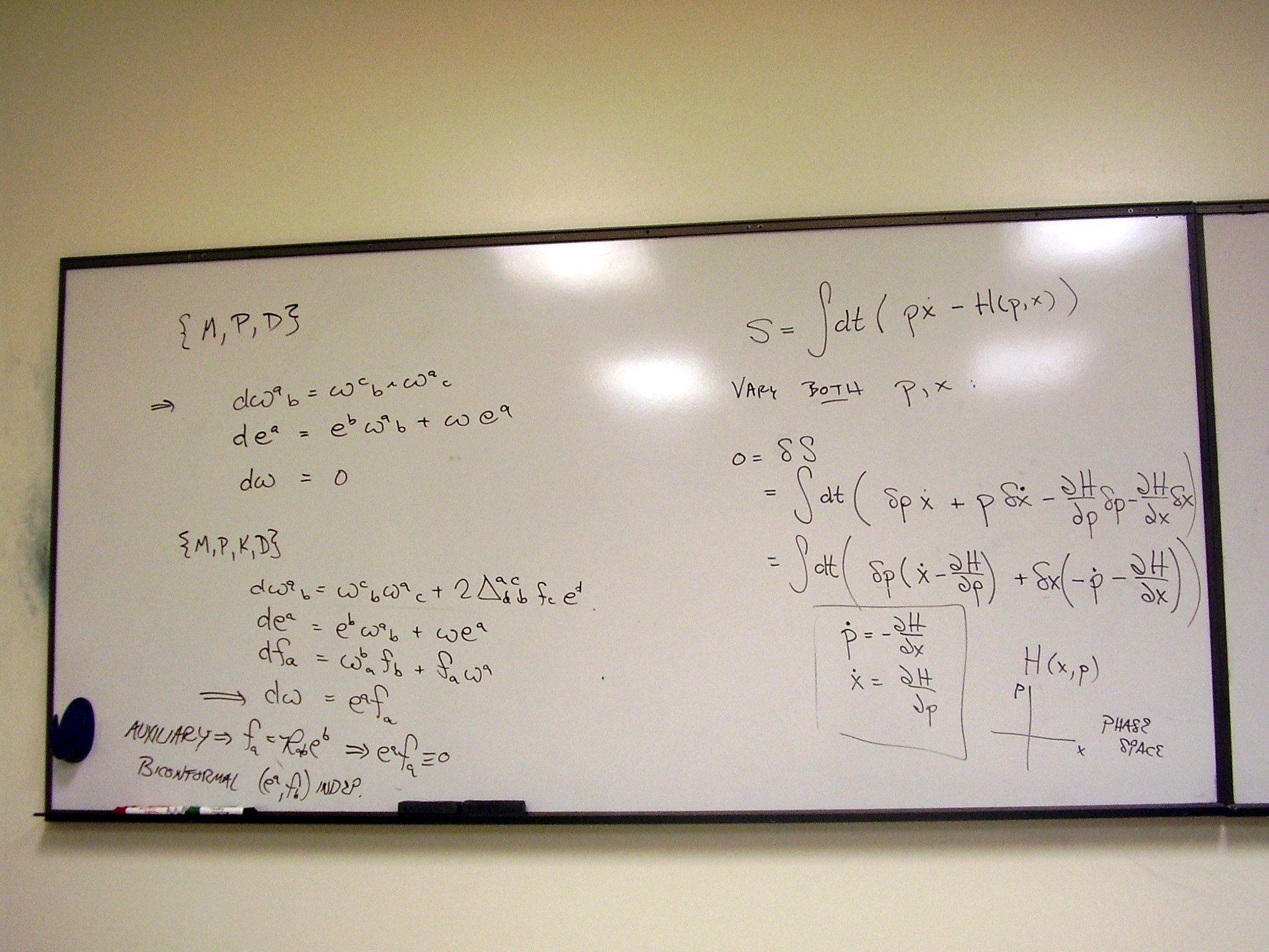
Friday, April 3, 2009
Lecture: Hamiltonian Mechanics
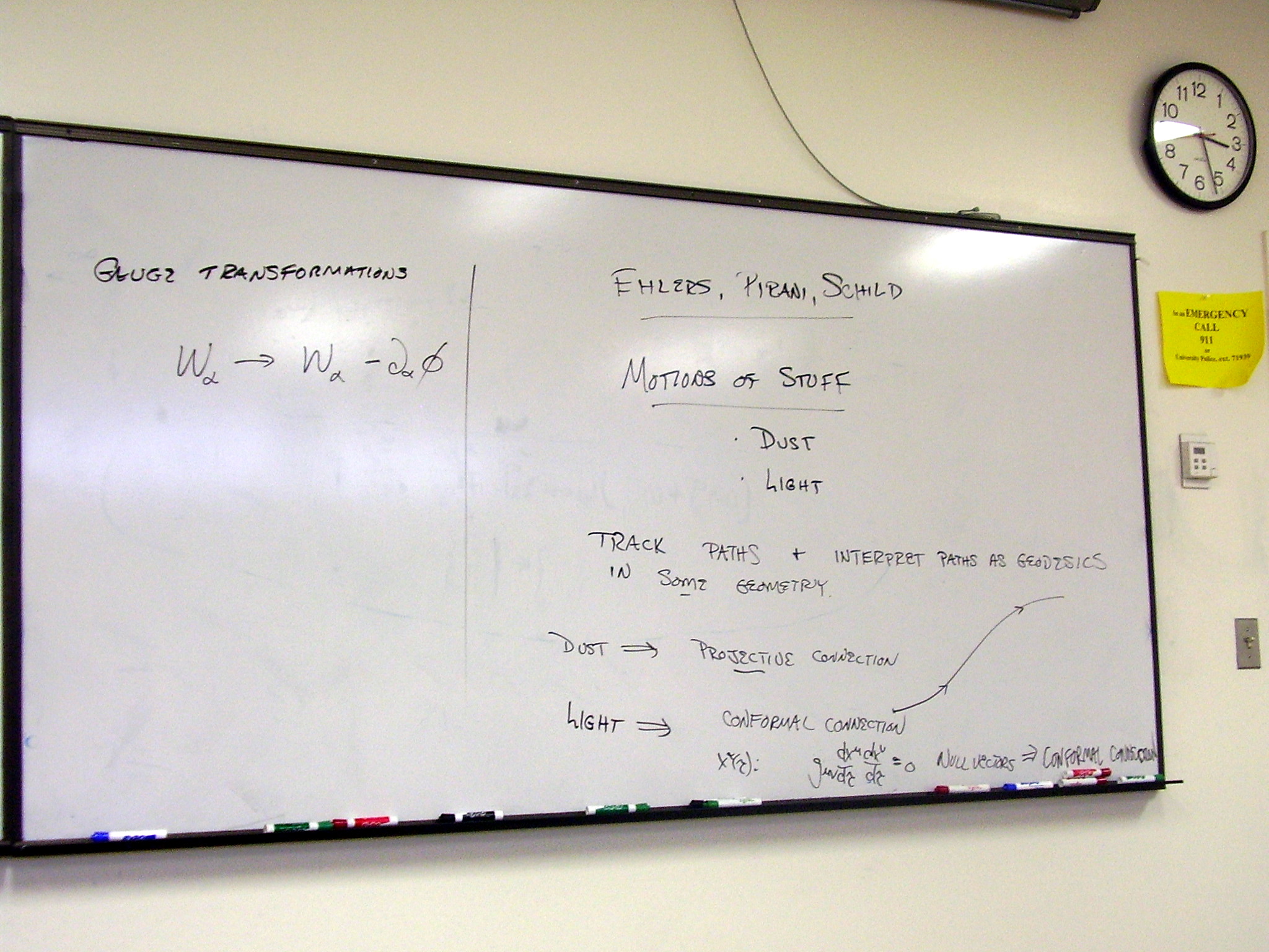
Gauge transformations of
connection 1-forms. Why the solder form becomes a tensor:
The 2nd Bianchi
identity in components:
The relationship between
the spin connection and the Levi-Civita (Cristoffel) connection:
The dilatational gauge
vector as the Lagrangian. Homothetic (Weyl) geometry.
The conformal Lie algebra:
Lagrange and Hamiltonian
dynamics; the action and its variation. Euler-Lagrange equation; Hamilton’s
equations:
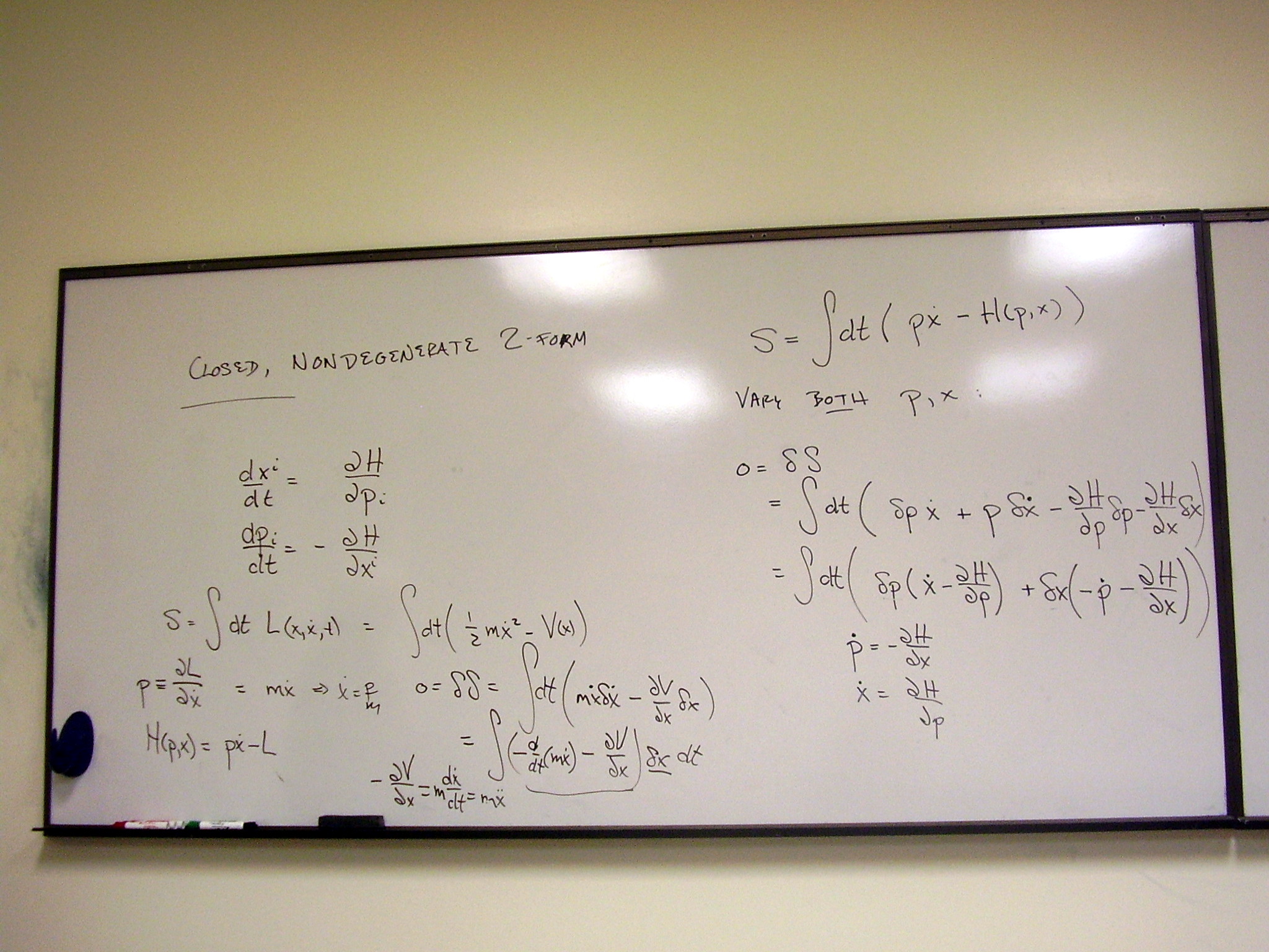
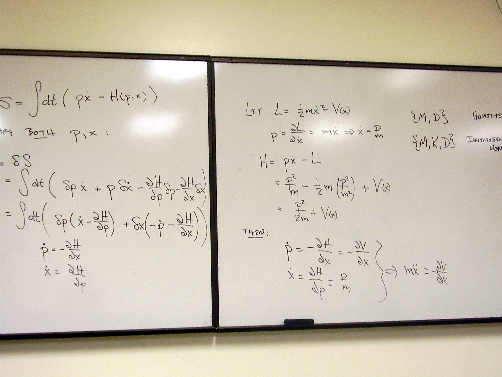
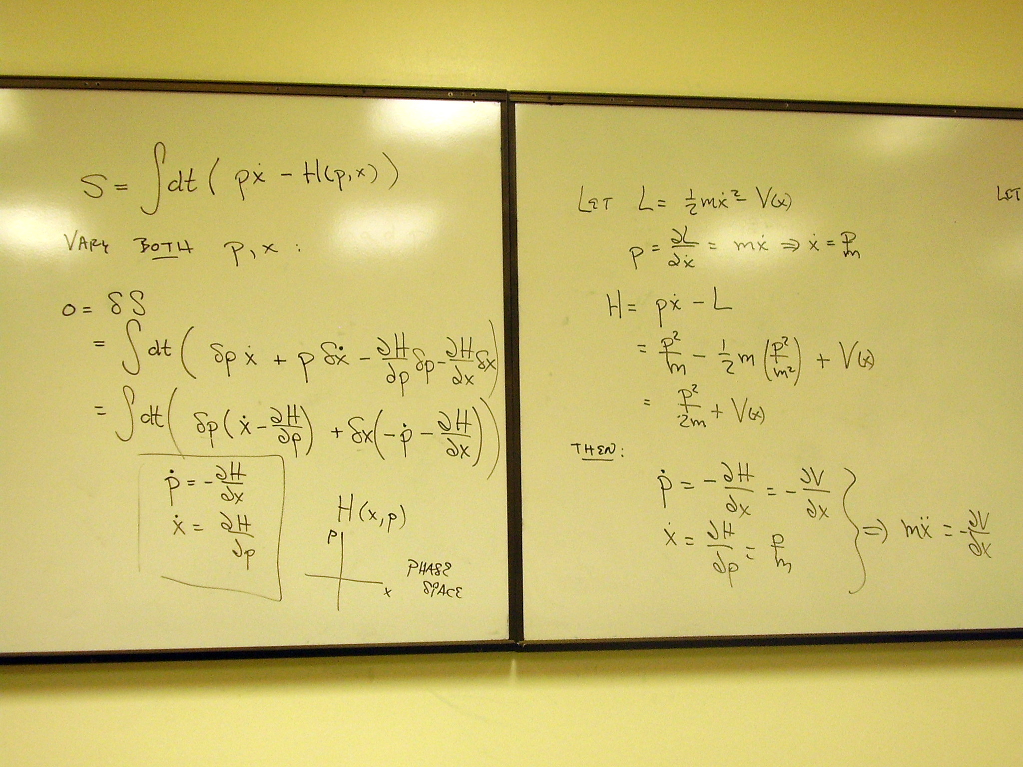
Unified phase space
coordinates and the symplectic form:
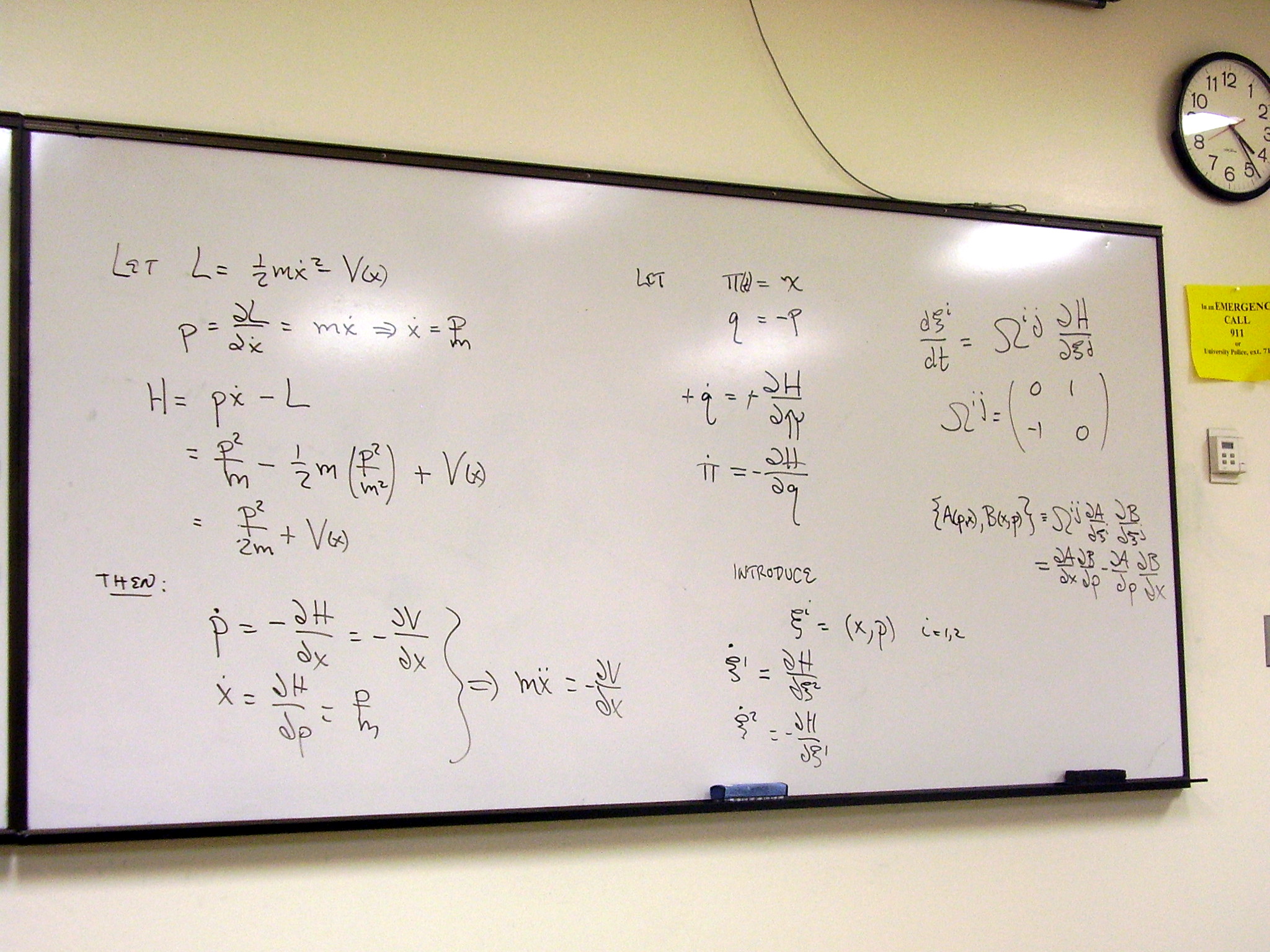
Poisson brackets:
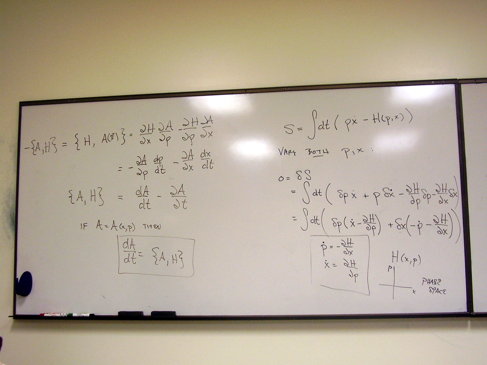
Comment on quantization:
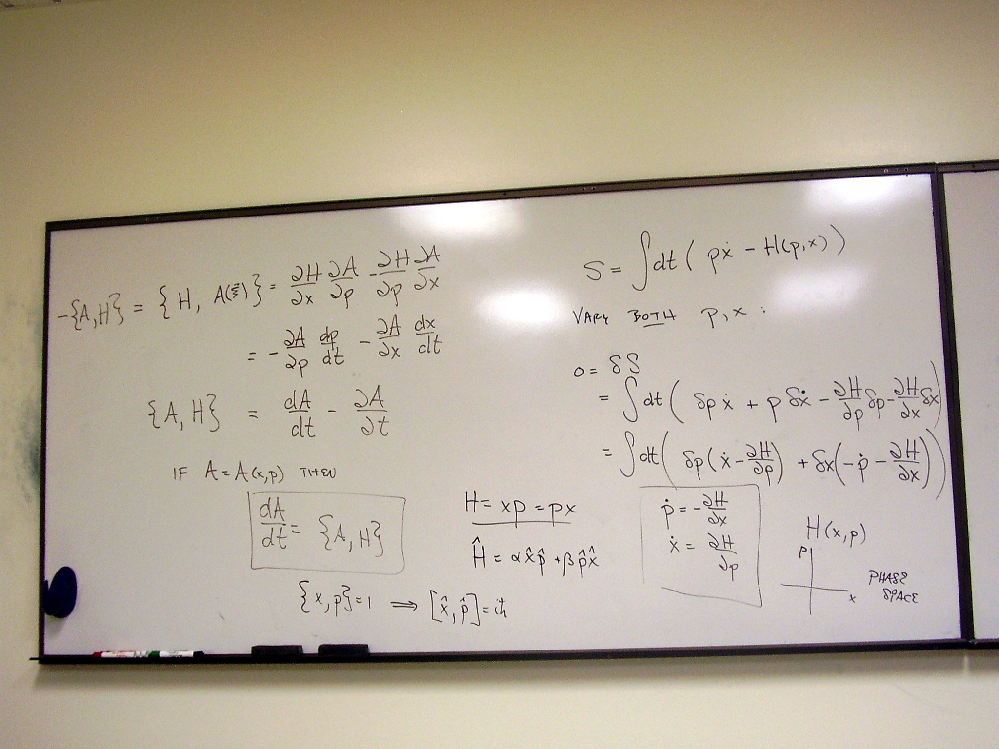
Conformal structure
equations; two gaugings of the conformal group:
Notes: April
Notes: Gauge
theories of gravity (Updated July 2; essentially complete)
Poincaré, Weyl, auxiliary
conformal and biconformal gauge theories.
Notes: Curvature-linear
action for biconformal gauge theory
Developing the action for
biconformal gravity.
Excerpts from:
WehnerS, Andre and Wheeler, James T., Conformal Actions in any dimension,
Nuclear Physics B 557 (1999) 380-406.
Also available online at: http://arxiv.org/pdf/hep-th/9812099
Notes: Solution
to the biconformal field equations (zero torsion)
The full solution to the
zero-torsion field equations arising from the curvature-linear action in
biconformal gauge theory.
Notes: Final version
of New
conformal gauging and the electromagnetic theory of Weyl
The first description of the
biconformal gauging in which the extra dimensions play an important role. Part,
but not all, of the Weyl vector is identified with the electromagnetic
potential.
Wheeler, J. T., New conformal gauging and the electromagnetic
theory of Weyl, Journal of Mathematical Physics 39 (1) (January, 1998) pages 299-328.
Also available online at: http://arxiv.org/pdf/hep-th/9706214
Notes: Final version
of Gauging
Newton's law
Hamiltonian dynamics as a
conformal gauge theory of Newton’s second law.
Wheeler, J. T., Gauging Newton’s Law, Canadian Journal of Physics, vol. 85, issue 4, pp. 307-344.
Also available online at: http://arxiv.org/pdf/hep-th/0305017
Notes: Final version
of Quantum
mechanics as a measurement theory on biconformal space
Quantum mechanics as a
measurement theory of biconformal geometry.
Anderson, L. B. and
Wheeler, J. T., Quantum theory as a biconformal measurement theory, Int. J.
Geom. Meth. Mod. Phys. 3 (2006) 315, (35pp.)
Also available online at:
http://arxiv.org/pdf/hep-th/0406159
|
|